
Variable Importance Analysis in Default Prediction using Machine
Learning Techniques
Başak Gültekin
and Betül Erdoğdu Şakar
Faculty of Engineering and Natural Sciences, Bahçeşehir University , Beşiktaş, Turkey
Keywords: Credit Scoring, Default Prediction, Feature Selection, Classification, Boruta, Logistic Regression, Random
Forest, Artificial Neural Network.
Abstract: In this study, different data mining techniques were applied to a finance credit data set from a financial
institution to provide an automated and objective profitability measurement. Two-step methodology was used
Determining the variables to be included in the model and deciding on the model to classify the potential
credit application as “bad credit (default)” or “good credit (not default)”. The phrases “bad credit” and “good
credit” are used as class labels since they are used like this in financial sector jargon in Turkey. For this two-
step procedure, different variable selection algorithms like Random Forest, Boruta and machine learning
algorithms like Logistic Regression, Random Forest, Artificial Neural Network were tried. At the end of the
feature selection phase, CRA and III variables were determined as most important variables. Moreover,
occupation and product number were also predictor variables. For the classification phase, Neural Network
model was the best model with higher accuracy and low average square error also Random Forest model
better resulted than Logistic Regression model.
1 INTRODUCTION
Financial institutions must work in accordance with
credible and clearly defined lending criteria. These
criteria should be sufficient to provide adequate
information about the structure of the borrower and
the credit, the purpose of borrowing, and the source
of the repayment. Financial institutions should
establish an independent and uninterrupted system
for the examination of loans and the results of such
examinations should be communicated directly to
the financial institutions management board and the
senior management.
In other words, it was aimed to create a credit
scoring model by examining the credit data. . Credit
scoring is a method of evaluating the credit risk of
loan applications. Using historical data and statistical
techniques, credit scoring tries to isolate the effects of
various applicant characteristics on delinquencies and
defaults. The purpose of measuring the credit risk is
to manage the loans with a portfolio approach, to
make the pricing risks, and to assure against
unexpected losses. Also, with the help of this study,
finance data was used to establish a high-power
model to assess the financial institutions individual
credit policy and to identify the default loan prediction
with the aim of increasing profitability and decreasing
the default risk.
While creating a model for internal rating
purposes, determining the variables to be included in
the model and the weighting of these variables in the
model is the main problem. In this study the risk
weights are analyzed by using multivariate statistical
analysis methods for estimation of default and not
default. By eliminating the missing and erroneous
data, a dataset consisting of 16.000 observations of 19
different variables obtained. SPSS tool was used to
draw data from the financial institutions’s system and
a table was created which has nearly 1.200.000
observations. 16.000 observations were randomly
selected by using SPSS tool from the obtained table,
taking care that the data is balanced.
Data set contains between March’2016 and
March’2017 data which belongs to individual loan
customers. Initially data analysis namely data
cleaning, missing value solutions, outlier detection
and visualization was done to make data clear to
anyone who has no idea about data analysis or mining.
Secondly relevance analysis made which contains
univariate analysis that examined each variable and
each variable with class variable and feature selection
was made. Variables which are more related to target
56
Gültekin, B. and ¸Sakar, B.
Variable Importance Analysis in Default Prediction using Machine Learning Techniques.
DOI: 10.5220/0006872400560062
In Proceedings of the 7th International Conference on Data Science, Technology and Applications (DATA 2018), pages 56-62
ISBN: 978-989-758-318-6
Copyright © 2018 by SCITEPRESS – Science and Technology Publications, Lda. All rights reserved

and have more power to measure default were selected
for modelling part of project.
2 DATASET DESCRIPTION
The dataset used in this study consists of 16000
samples each represented with a feature vector of 18
variables and an associated class label. The variable
names and types along with their ranges are shown
in Table 1. The dataset belongs to the individual loan
applications of a financial institution.
The variables can be categorized under 2 main
categories which are finance-related information and
personal information. In this section, we briefly
introduce the input variables under these 2 categories
and the class variable to clarify the information
represented by each variable in our dataset.
2.1 Finance-related Information
The variable denoted with ‘housingMaturity’ in Table
1 represents for how many months the customer is
paying the instalments of housing credits. The
maturity value of housing credits can take a value
between 6 and 240 months in Turkish finance system.
Similarly, vehicle maturity shows the number of
months for the credit instalments of vehicle loan. This
is also an integer variable and has a range from 0 to 60
months. The number of months for the credit
instalments of consumer loan is stored in the
consumer maturity variable, which has a range from 0
to 120. The variable referred to as ‘ProductNumber’
in Table 1 represents the total number of different
products taken by the customer before, including the
current active loan. This variable is in integer type
and it has a range from 1 to 113. The ‘workingTime’
and ‘workplace’ variables show the term of
employment and status of the working place of the
credit customer, respectively.
While the working time information is represented
with an integer variable, the workplace is a categorical
variable which takes 3 different values as “Public”
“Private or Corporate” and “Other”. The other
variable related with the working place of the
customer is ‘Ownership’ which is a categorical
variable and takes 4 different values indicating the
owner of the workplace the customer is working for.
The possible values of this variable are “personal”,
“rental”, “family-owned” and “other”. The
‘insuranceCode’ variable represents the type of social
security of the credit customer. It is a categorical
variable which can take 5 different values.
Loan Type is an indicator for consumer maturity,
vehicle maturity and housing maturity variables. It is
a factor variable and it is kept in financial institution’s
system in integer type. Variable has values as
“consumer loan”, “housing loan”, and “vehicle loan”
and kept as 1, 2, and 3 in the system. The financial
institution is using this variable for analyzing the
relationship between the number of instalments and
whether the credit will end as default or not default.
Most of the credits given by the financial institution
are consumer credits rather than housing and vehicle.
There is a "due date" in every kind of credit
settlements as credit card, credit deposit account or
different loan types. If the payment due date is 1 or 2
days delayed, the delay is referred as 1 term. If
consecutive loan repayments have been made late on
a two-time payment date, it is a two-term delay. The
“DefaultNumber” variable refers to customers who
have experienced the legal default process before. The
credits whose repayment period is delayed for 3 terms
go into default process and closed after completion of
repayment.
There are 2 important credit scores determined by
the Consumer Reporting Agency (CRA) for each
customer. One of these variables, referred to as CRA
in Table 1 is an integer variable with a range from 0
to 1612. The CRA calculates this value according to
their internal rating system and provides to the
financial institution when required. The value of 0
(zero) means that the score cannot be calculated by
CRA for that customer. The higher the score the more
credit worthiness customer has. The other important
credit score included in our dataset is the individual
indebtedness index (III) which is designed to predict
the risks arising from high indebtedness. The main
difference between CRA score and III value is that
while the CRA value aims to determine the risk based
on the past or current payment problems, III value is
used to identify people who have not suffered any
difficulties but are likely to suffer in the future due to
excessive borrowing.
2.2 Personal Information
In addition to the variables related with the financial
status of the customers, the dataset contains some
personal information that might be important in the
credit worthiness of the customer. These are marital
status, occupation, education status, and age.
The marital status variable specifies the marital
status of the customer as of the date of credit
application. This is a categorical variable with 5
different values. The occupation information is
represented with 8 different categories each one
Variable Importance Analysis in Default Prediction using Machine Learning Techniques
57
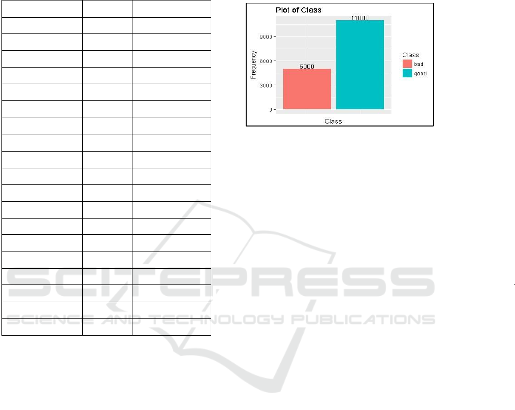
Table 1: Variables of the credit scoring dataset used in this
study.
Variable Name
Type
Range
housingMaturity
interval
[0-180]
maritalStatus
categorical
[1,2,3,4,5]
occupation
categorical
[1,2,3,4,5,6,7,8]
educationStatus
categorical
[0,1,2,3,4,5,6,7,8]
vehicleMaturity
interval
[0-60]
consumerMaturity
interval
[0-120]
ProductNum
interval
[0-113]
workingTime
interval
[0-14556]
workplace
categorical
[0,1,2]
OwnershipCode
categorical
[0,1,2,3]
age
interval
[18-85]
insuranceCode
categorical
[0-99]
CRA
interval
[0-1612]
III
interval
[0-64]
loanType
categorical
[1,2,3,4]
D2
interval
[0-18]
defaultNum
interval
[0-6]
D1
interval
[0-10]
class
target
[0,1]
corresponding to a profession. The education status
variable is an ordinal variable showing the level of
education of the customer. This variable can take 9
different values and its value is determined based on
the most recently graduated educational institution of
the customer. The other personal information is the
age of the customer as of the date of credit application
and it has a range from 18 to 85.
2.3 Class
The target variable of the data set is referred to as
“Class” in Table 1 which represents whether a credit
is gone into default or not. Hence, the learning
problem in this study is a binary classification
problem in which the input variables are mapped to
an output which takes one of the two discrete values.
The distribution of the class labels is shown in
Figure 1. According to the regulations of the Banking
Regulation and Supervision Agency (BRSA), if a
credit card debt or a loan payment is overdue for 90
days, the financial institiution has the authority to
initiate legal proceedings for debt collection. This is
called “default” in banking terminology.
Figure 1: Distribution of the class variable.
3 DATA ANALYSIS AND
VISUALIZATION
In this section, we present a detailed analysis of the
finance-related and personal variables of our dataset.
The variables that possess information about the
financial status of the customer and the details of the
credit are considered to be effective in default
prediction. A small amount of the credits, 782 out of
16000 (4.88%), is of type housing credit. As seen in
Figure 2, the probability that the loan will default at
the beginning of the loan payment is higher and it
tends to decrease in time.
Most of the samples in our dataset, 13298 out of
16000, belong to consumer credit type. According to
the regulations of BRSA, the maturity of the consumer
loan is limited to 48 months. However, the maturity
can be extended up to 120 months in case of
mortgaging a property, dwelling, or workplace. As it
is seen from Figure 3, like housing maturity, the
probability that a consumer loan will default decreases
in time. The box plot of vehicle loan is not shown
since it constitutes a small portion of the dataset (63
out of 16000). The maturity information of the other
credit type, credit card and overdraft account shown
as ‘kk-kmhkh- kmh” in Figure 4, in our dataset is not
available since it is a checking account.
According to the BRSA regulations, if the
minimum payment amount of the credit is not paid
within 90 days after the expiry date, the legal follow-
up process is started by applying default interest.
Figure 4 shows the number of default loans in the
previous financial history of the consumers by loan
type. As it is seen, most of the customers do not have
any default loan before.
DATA 2018 - 7th International Conference on Data Science, Technology and Applications
58
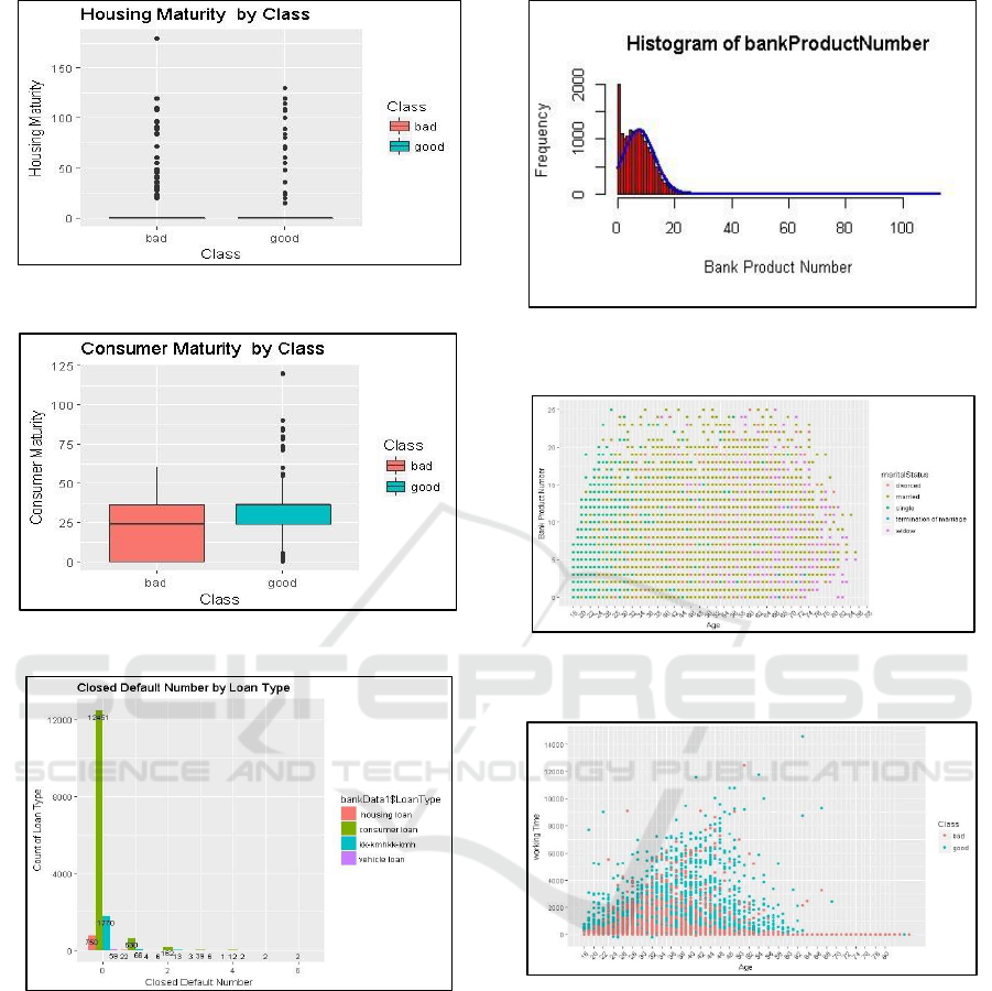
Figure 2: Boxplot of the housing maturity variable.
Figure 3: Boxplot of the consumer maturity variable.
Figure 4: Number of previous defaults for each loan type.
The product number variable is left-skewed as
shown in Figure 5. The number of customers using
more than 25 products in our dataset is 95 only
(%0.95) of the dataset. These extreme values are
marked as outliers using the quartile-based outlier
detection approach and excluded from the dataset.
Figure 6 shows the distribution of number of
products by age and marital status variables. As it is
seen, the middle aged and married customers are
likely to use more banking products than the other
profiles.
Figure 5: Histogram of the number of products each
customer had used before.
Figure 6: Distribution of number of products according to
age and marital status.
Figure 7: Class distribution with respect to age and work.
Figure 7 shows the class distribution with respect
to age and working time variables. It is seen that the
customers with a longer period of working time are
less likely to have defaults.
4 FEATURE SELECTION AND
DATA PREPROCESSING
Feature selection is an important task in predictive
modelling. One of the benefits of feature selection is
to improve the performance of the prediction model
Variable Importance Analysis in Default Prediction using Machine Learning Techniques
59
by alleviating the curse of dimensionality problem
(Tsai, 2009). Besides, ranking the features according
to their importance in the predictive model reveals
some important domain-specific information which
can be helpful for the experts of that sector. In this
section, we perform effective feature selection
algorithms called Boruta (Kursa and Rudnicki, 2010)
and Random Forest (Breiman, 2001) to select a
minimal subset of variables which, when used
together, have a great influence in the prediction of
default credits. Boruta is a wrapper feature selection
algorithm which is based on random forest variable
importance measure (Kursa and Rudnicki, 2010). The
intuitive idea behind Boruta is that it finds comparing
the importance of original variables with the
importance of their randomly shuffled copies and
choosing the variables with higher importance than its
shuffled copies. The shuffled copies added to the
original dataset are called shadow features. The
Boruta algorithm can be stopped when a predefined
number of random forest runs. Another alternative
stopping criterion is to obtain a label, “important” or
“unimportant”, for each of the variable in our dataset.
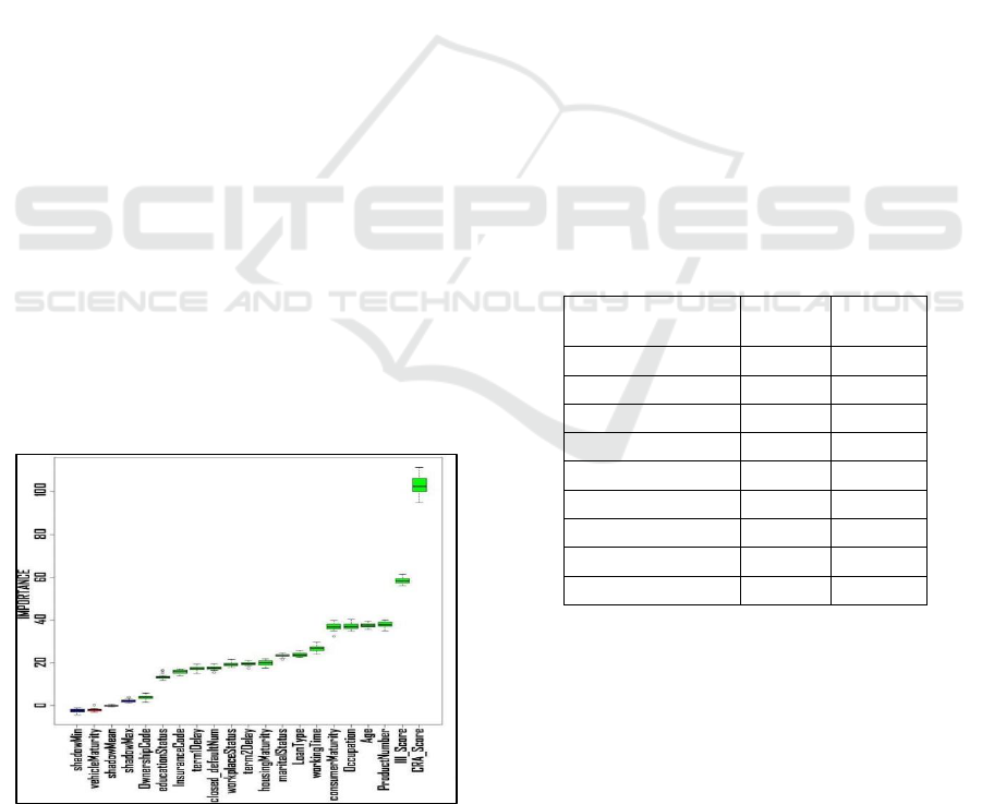
Figure 8 shows the importance level of each variable
found by Boruta algorithm. It is seen that the CRA
score of the customer is the most important variable in
the prediction of the default credits. The other scoring
variable in our dataset, III, has been found to be the
second important variable. These results show that the
scores computed by the relevant organizations are
important indicators of default prediction. Boruta is a
wrapper algorithm that also takes the redundant
information among the variables about the target
variable. In other words, the Boruta algorithm
evaluates the importance of variables when used
together for the target variable prediction. This shows
Figure 8: Importance level of input variables found by
Boruta algorithm
that CRA and III values carry important and
complementary information about the default credits.
As seen in Figure 8, the CRA and III variables are
followed by another financial status-related variable
which is the number of products used by the customer.
The next two important variables are about occupation
and age which constitute personal information that
contain indirect information about the financial status
of the customer. Another personal information which
represents the marital status of the customer is ranked
at 9
th
position.
According to the importance levels seen in Figure
8, while CRA and III values can be considered in the
highest level of importance, the next four variables
which are “productNumber”, “age”, “occupation” and
“consumerMaturity” can be grouped in the next level
of importance with very close important levels. The
boxplot analysis show that the importance levels of
these variables are not statistically significant from
each other. These four variables are followed by three
variables with similar importance values which are
“workingTime”, “loanType” and “maritalStatus”.
Therefore, we exclude the remaining variables from
the dataset and establish the prediction model with the
top-ranked 9 variables which have higher importance,
i.e. mean impurity values higher than 20. The selected
variables along with their minimum impurity values
found by Boruta algorithm are shown in Table 2.
Table 2: Selected variables using Boruta algorithm.
Variable Name
Mean
Impurity
Minimum
Impurity
CRA
102.9
94.9
III
58.4
56.1
productNumber
38.0
35.1
Age
37.6
35.7
Occupation
37.2
34.8
consumerMaturity
36.8
32.4
workingTime
26.7
23.9
loanType
23.8
22.6
maritalStatus
23.4
17.7
In Figure 9, the histograms of the most effective
four continuous variables are presented. The
histogram of the number of products each customer
uses has already been shown in Figure 5. As it is seen,
CRA, which has been found as the most effective
variable in feature selection step, is right skewed.
Therefore, we apply a logarithmic transformation to
this variable. On the other hand, the “ProductNumber”
and the “workingTime” variables are left skewed as
seen in Figure 5 and Figure 9, respectively. We have
also applied logarithmic transformation to these
DATA 2018 - 7th International Conference on Data Science, Technology and Applications
60

variables and fed to the prediction algorithms using
the transformed variables. As a result, 9 of the original
input variables provided with their description in
Table 1 are eliminated after the feature selection
process and the remaining 9 variables are chosen to be
included in the prediction model.
Figure 9: Histograms of selected four continuous variables.
5 CLASSIFICATION
In this section, we feed the selected variables as input
to three machine learning algorithms and present the
classification performances of each algorithm. The
most commonly used algorithm in default prediction
is logistic regression (Hosmer, et al., 2013) since it is
a simple, linear and easy to explain algorithm which
is one of the important requirements of this problem
(Hilbe, 2014). In addition to logistic regression, we
also apply multilayer perceptron (West, 2000) and
random forest algorithms (Brown and Mues, 2012)
which are capable of capture the non-linear
dependencies between the variables and the target
variable.
We split the dataset into two partitions and use
70% of the data to train each model. The rest 30% of
the samples are used for validation. In logistic
regression, the output is passed through a sigmoid
function which converts its numerical output to a
probability estimate. In the default prediction
problem, we have two classes, default or not-default.
The logistic regression used for binary class is called
binomial logistic regression. The obtained
probability estimates after passing the output through
sigmoid function represents the likelihood of that
credit going into default.
All variables have been found to be significant at
p_value 0.05 level according to the results of logistic
regression algorithm. This shows that the features
selected by the Boruta feature selection algorithm are
related with the default information.
The results obtained on validation set with each of
the classifier used in this study are shown in Table 3.
It is seen that logistic regression performed worse than
multilayer perceptron (MLP) and random forest. The
dataset used in this study cannot be termed as an
imbalanced dataset since the class distribution is 37%
to %63. However, it is also not uniform distribution.
Therefore, in addition to the accuracy metrics, we
provide the AUC value.
The neural network architecture used in this study
is a multilayer perceptron with a single hidden layer.
As shown in Table 3, the highest accuracy, TPR and
AUC are achieved with multilayer perceptron. The
AUC results also show that MLP gives more balanced
performances on positive and negative instances than
logistic regression.
The random forest algorithm is an ensemble
learning algorithm which creates multiple trees hence
called “forest”. In binary classification, a majority
voting or stacking approach is used to combine the
predictions of the trees. In this study, we use voting
mechanism to produce the final output of the forest.
Table 3 shows that random forest gives better results
than logistic regression in terms of both accuracy and
AUC. The performance of random forest is close to
that of MLP.
Figure 10: ROC charts of three models.
Determining a bad credit beforehand is more
important than to allocate good credit in banking.
Hence, to measure performances of models, we
applied ROC which summarize classifier performance
over a range of tradeoffs between true positive and
false positive error rates given by AUC.
Table 3: Classification performances of each classifier on
validation set.
Classifier
Accuracy
TPR
AUC
Logistic
Regression
0.812
0.783
0.734
Multilayer
Perceptron
0.847
0.792
0.832
Random
Forest
0.842
0.788
0.823
Variable Importance Analysis in Default Prediction using Machine Learning Techniques
61

It is seen from Figure 10 random forest and neural
network has similar ROC charts and better than
logistic regression.
6 CONCLUSIONS
This study includes comparative analysis of PD
production based on credit scores and grading
methods which must be applied compulsorily in all
banks in accordance with Basel standards and
applying machine learning algorithms to improve the
score model.
Actual customer data is used in the study. Since
the actual data is the subject, each variable should be
analyzed separately from the business perspective in
the univariate analysis. In some cases, according to the
statistical management analyses, the values accepted
correctly may not be regarded as correct from the
business point of view.
According to analysis most customers of the
financial institution are retired category. There is a
positive relation between the customer receiving their
salaries from same financial institution and not
defaulted credit.
Encouraging retiree clients to get their salaries out
of this financial institution may be an accurate step in
terms of credit profitability would be a conclusion.
Housing Maturity, Vehicle Maturity, Consumer
Maturity, Workplace, Ownership Code, Insurance
Code, Term 1 Delay, Education Status and Marital
Status are not the strong explanatory variables of
credit default. KKB_score variable is a strong
explanatory variable in both models. “default credit”
and “d2” variables are also strongly determining the
dependent variable. Due to make a robust model it
may be a way to increase the weights of these
variables to calculate the predicted default value.
At the same time, some conclusions can be drawn
about the banking and credit policy. Occupation
variable is a powerful predictor variable for Class
variable. Therefore, different marketing studies can be
done for different occupational groups and new
customers with lower risk groups can be tried to gain.
Also, since ProductNumber is an important variable
the bank may create marketing efforts and different
collateral schemes according to different age and
occupational groups using different product groups.
As a result, the results of the experimental work
presented here is used in real life for a specific
financial institution in Turkey.
REFERENCES
Breiman, L., 2001. Random Forests. 45(1), pp. 5-32.
Brown, I. & Mues, C., 2012. An experimental comparison
of classification algorithms for imbalanced credit
scoring data sets. Expert Systems with Applications,
39(3), pp. 3446-3453.
Hilbe, J. M., 2014. Logistic Regression. s.l.:Springer-Verlag
Berlin Heidelberg .
Hosmer, D. W., Lemeshow, J. S. & Sturdivant, R. X., 2013.
Introduction to the Logistic Regression Model. s.l.:John
Wiley and sons,Inc.
Kursa, M. B. & Rudnicki, W. R., 2010. Feature Selection
with the Boruta Package. Journal of Statistical
Software, 36(11).
Tsai, C.-F., 2009. Feature selection in bankruptcy
prediction. 22(2), pp. 120-127.
West, D., 2000. Neural network credit scoring models.
Computers and Operations Research, 27(11-12), pp.
1131-1152.
DATA 2018 - 7th International Conference on Data Science, Technology and Applications
62
