Analysing Team Formations in Football with the Static Qualitative

Trajectory Calculus

Jasper Beernaerts

, Bernard De Baets

, Matthieu Lenoir

, Kristof De Mey

and Nico Van de Weghe

CartoGIS, Department of Geography, Ghent University, Krijgslaan 281 (S8), 9000 Ghent, Belgium

KERMIT, Department of Data Analysis and Mathematical Modelling, Ghent University,

Coupure links 653, 9000 Ghent, Belgium

Department of Movement and Sports Sciences, Ghent University, Watersportlaan 2, 9000 Ghent, Belgium

Keywords: Football, Team Formation Analysis, QTC, Sports Analytics.

Abstract: In this paper, we introduce the Static Qualitative Trajectory Calculus (QTC

), a qualitative spatiotemporal

method based on the Qualitative Trajectory Calculus (QTC), for team formation analysis in football. While

methods for team formation analysis are mostly quantitative, QTC

enables the comparison of team

formations by describing the relative positions between players in a qualitative manner, which is much more

related to the way players position themselves on the field. To illustrate the method, we present a series of

examples based on real football matches of a 2016-2017 European football competition. With QTC

, team

formations of both an entire team as well as a smaller group of players can be described. Analysis of these

formations can be done for multiple matches, thereby defining the playing style of a team, or at critical

moments during a game, such as set pieces.

1 INTRODUCTION

In this paper, we introduce a new method for

analysing team formations in football, based on the

Qualitative Trajectory Calculus (QTC; Van de

Weghe, Cohn, et al., 2005). We start by giving a brief

overview of established methods for analysing team

formations in popular team sports and football more

in particular. After that, we present the static QTC

(QTC

), an extension of the calculus introduced by

Van de Weghe et al. in 2005. After presenting the

novel methodology, we illustrate the application of

QTC

for analysing team formations in football by a

series of real football examples. In the fifth section,

we discuss the applicability of the method, its

drawbacks and opportunities, before ending with a

conclusion.

2 STATE OF THE ART

Thriving on technological advances in tracking

technology and the opening up of different sports

branches to data gathering, sports analytics has

become a booming business in recent years (D’Orazio

and Leo, 2010). Dozens of parameters from players,

such as speed, heart beat rate, transpiration level,

position, acceleration, jump height, goals scored,

attempts, tackles, etc. are being monitored during

training and matches of different sports. Even data at

team level, called collective variables, such as

formation, pass statistics, average positions, number

of shots and others are being gathered (Rein and

Memmert, 2016). In this overview, we will focus on

collective variables and more specifically on the

analysis of spatial formations in team sports, which

we will refer to as ‘team formation analysis’ in the

remainder of this paper. Since almost all team

formation analysis methods, regardless of the sport,

use positional data of the players, we start by giving

a brief but focused overview of the state of the art of

team formation analysis in popular sports, before

providing a broader overview of the domain for

football. For a more general overview of all different

sports analytics methods in football, we refer to the

works of Rein and Memmert, 2016 and Memmert et

al. (2017).

Beernaerts, J., Baets, B., Lenoir, M., Mey, K. and Weghe, N.

Analysing Team Formations in Football with the Static Qualitative Trajectory Calculus.

DOI: 10.5220/0006884500150022

In Proceedings of the 6th International Congress on Sport Sciences Research and Technology Support (icSPORTS 2018), pages 15-22

ISBN: 978-989-758-325-4

2.1 Team Formation Analysis

In American football, Atmosukarto et al. (2013) did

efforts for the automatic recognition of offensive

team formations, which they defined as “The spatial

configuration of a team’s players before a play starts”

(Atmosukarto et al., 2013, p. 1) Their method

automatically detects when one of five reference

offensive team formations is achieved during the

game. The big difference with football, however, is

that a football game is more fluent and dynamic, thus

team formations tend to change more during the

course of the game (Atmosukarto et al., 2013). Team

formation analysis in volleyball has been conducted

by Jäger and Shöllhorn (2012). Because of the distinct

separation of a volleyball game in separate rallies,

Jäger and Shöllhorn used the positions of the players

at the start and end of the rallies instead of the average

positions during the rallies. Furthermore, they divided

the players into attacking and defensive groups,

analysing the shape of the two groups separately. On

top of that, they discovered that, given a dataset with

formations of six teams, an unknown team formation

could be correctly classified/assigned to one of the six

teams. In basketball, Lucey et al. (2014) analysed

defensive team formations of basketball players in the

three seconds leading to a three-point shot attempt,

finding they were able to predict whether the team

was going to give up open shot opportunity or not.

At this point, we would like to stress the

difference between team formation analysis, which is

the topic of this paper and is a spatial type of analysis,

and the analysis to choose the optimal line-up of a

team, which can benefit from player-specific data.

The latter type of analysis focuses on the selection of

actual players for each of the positions on the field

and has been investigated more rigorously in, for

example, hockey (Colleen Stuart, 2017), football

(Barrick et al., 1998; Tierney et al., 2016), volleyball

(Boon and Sierksma, 2003), basketball (Dezman et

al., 2001) and cricket (Ahmed et al., 2013).

2.2 Team Formation Analysis in

Football

In football, teams generally aim to play according to

a specific team formation (Kaminka et al., 2003;

Kuhlmann et al., 2005), which can be defined as “A

specific structure defining the distribution of players

based on their positions within the field of play”

(Ayanegui-Santiago, 2009, p. 1). Advantages of one

specific team formation with respect to others, e.g.

increased running distances when playing against a 4-

2-3-1 instead of a 4-4-2, have been described by

Carling (2011). Mapping the advantages of different

team formations can be useful when comparing them

with the own team strengths and weaknesses in order

to choose the most suitable team formation for a

game. Team formation analysis in football can be

performed in various ways, based on different key

performance indicators that are derived from the

players’ positions (Memmert et al., 2017). For

example, Sampaio and Macãs (2012) suggested the

team centroid, team entropy, a team stretch index and

the surface area of the team as key performance

indicators for team formation analytics. Going further

on this, Frencken et al. (2012) added the inter-team

distance, i.e. the distance between the centroids of

both teams, as a key performance indicator to detect

goals or attempts in a match. Lemmink and Frencken

(2013) demonstrated the possibility to use these key

performance indicators not only for the entire team

but also for subsets of the team such as players with

specific roles, e.g. attackers or defenders.

A method for automatic detection of the type of

team formation based on the average position of the

players was proposed by Bialkowski et al. (2014).

They argue that, because of the players swapping

positions during the game, static ordering of the

players does not accurately represent the team

formation. In order to cope with this, they introduce

dynamic ordering of players by the role that they

occupy at a given instant in time. Using data from a

whole Premiere League season, Lucey et al. (2013)

and Biakowski et al. (2014) found no significant

difference between formations of different teams, but

could detect that English Premier League teams used

more offensive team formations during home games.

Various new methods use principles of (artificial)

neural networks (McCulloch and Walter, 1943).

Visser et al. (2001) used artificial neural network

systems to recognize the team formation of the

opponent team. Starting with the positions of the

opponent players at a certain timestamp, the neural

network tried to classify that moment into a set of

predefined team formations (Atmosukarto et al.,

2013) later used an analogue method in American

football) and proposed the appropriate counter team

formation for the own team. Going further on this

work, Ayanegui-Santiago (2009) proposed to include

multiple relations between players for the recognition

of team formations. He divided the players into three

groups (defenders, midfielders and attackers) and

used labelled graphs between nodes of adjacent

groups to describe and compare team formations.

The methods mentioned above generally aim at

calculating frequencies of team formations. This

facilitates comparison of different team formations

icSPORTS 2018 - 6th International Congress on Sport Sciences Research and Technology Support

and the temporal evolution of these team formations

during the game (Grunz et al., 2012). Furthermore,

the occurrence of team formations can be linked to

scoring goals and winning games, thus measuring the

success of a specific team formation for a team.

However, while most methods use quantitative

metrics, Perin et al. (2013) argue that quantitative

analysis is not sufficient to understand the team

formation of a game or a whole season.

Unfortunately, qualitative team formation analysis in

football is currently mostly performed by human

experts and is thus very labour intensive (Bialkowski

et al., 2014). The goal of this paper is to contribute to

this domain, by introducing QTC

for (automatic)

team formations analysis in football.

3 METHODOLOGY

In this section, we introduce the novel methodology

for sports team formation analytics. We start by

giving a brief overview of QTC, followed by the new

variant (QTC

) that was created for this type of

research. Following, we present a series of possible

applications for the method in team formation

analysis in football.

3.1 The Qualitative Trajectory

Calculus

QTC is a qualitative calculus for describing

spatiotemporal relations between two or more

Moving Point Objects (MPOs). The most basic

variant of the calculus, QTC

, describes the

movement of a pair of MPOs during a time interval

by means of two QTC-characters (Van de Weghe,

Cohn, et al., 2005). Afterwards, multiple variants of

QTC were introduced, each named by adding the

initial(s) of the variant’s name to the abbreviation

‘QTC’ in subscript (Bogaert et al., 2007; Mavridis et

al., 2015).

3.2 QTC

While QTC typically describes movement between

multiple objects, it can be extended easily to a new

variant named QTC

(Static Qualitative Trajectory

Calculus), which describes static formations of point

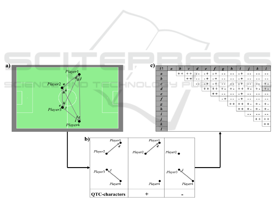
objects (POs), which are players in our case. When

describing the formation of POs with QTC

, the lack

of movement is dealt with by constructing all possible

vectors between the POs (Figure 1a). Subsequently,

QTC

-relations between each pair of vectors are

Figure 1: A formation of four players (POs) on a football field at t

and the vectors between them (a). The construction of the

QTC

-relations between two vectors d and l, consisting of the QTC

-relation of vector d with respect to the starting point of

vector l and of the QTC

-relation of vector l with respect to the starting point of vector d. If the vector moves away from the

starting point of the other vector, the QTC

-relation is denoted by ‘+’, if the movement is towards it, the QTC

-relation is

denoted by ‘-’. If the movement is neither away nor towards the marker (thus perpendicular to the connecting line between

the two starting points), the QTC

-relation is denoted by ‘0’ (b). The QTC

-matrix describing the full formation of the four

players, including all relations between all of the vectors (c).

Analysing Team Formations in Football with the Static Qualitative Trajectory Calculus

constructed similar to QTC

(Van de Weghe, Cohn,

et al., 2005), shown in Figure 1b for the vectors d and

l. The different QTC

-relations are stored in a QTC

matrix, where the first character in each cell is the

QTC

-relation of the vector in the row header with

respect to the vector in the column header, the second

character is the QTC-relation of the marker in the

column header with respect to the marker in the row

header (Figure 1c).

3.3 QTC

for Team Formation Analysis

By constructing a QTC

-matrix at different

timestamps, QTC

can be used to describe the team

formation at different moments in time. If the number

of players in the formation is identical at each of those

timestamps, the QTC

-matrices will have the same

dimensions and can be compared by calculating the

distance between them. The distance between two

QTC

-matrices is calculated by summing up the

pairwise distances between all of its elements (QTC

relations), thereby using the conceptual distance

between QTC-relations (Van de Weghe and De

Maeyer, 2005). By dividing the total distance

between two QTC

-matrices by the maximal possible

distance (depending on the matrix dimensions), the

relative distance is calculated. For easier

understanding, the relative distance is recalculated to

a similarity value between 0 and 1. The current

implementation of the methodology was done in the

Python programming language.

4 APPLICATIONS OF QTC

FOR

TEAM FORMATION ANALYSIS

IN FOOTBALL

In this section, we present a series of examples of the

QTC

-methodology for team formation analysis in

football. Considering the novelty of the method and

the lack of a good ground truth (Feuerhake, 2016), the

focus in this section primarily lies on introducing

rather than validating the results. All examples are

based on real football matches of a 2016-2017

European football competition, but are presented

anonymously for privacy reasons.

4.1 Full Team Formation

Often, trainers aim to use one or more predefined

team formation(s) for their field players (excluding

the goal keeper) according to the situation in the game

and the team formation of their opponent. By using

QTC

to describe both the desired team formation(s)

as well as the actual performed formation, an

evaluation of the team performance can be made.

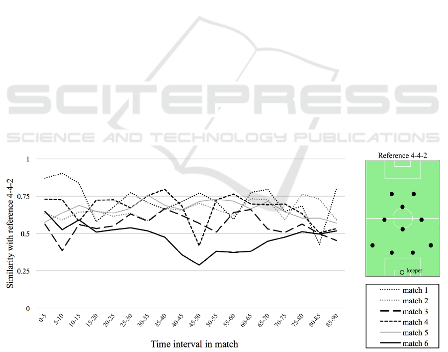
Figure 2, for example, shows compliance (similarity)

of an anonymous team with a 4-4-2 team formation

during six different matches, analysed with a

temporal resolution of five minutes. The higher the

similarity in the graph, the more the actual team

formation resembled the theoretical 4-4-2 shown on

the right side, during the game.

Figure 2: Similarity of an anonymous team with a theoretical 4-4-2 formation during 6 matches, with a temporal resolution

of 5 minutes.

icSPORTS 2018 - 6th International Congress on Sport Sciences Research and Technology Support

4.2 Analysis of a Teams Playing Style

While in Section 4.1 similarity with one reference

team formation is calculated, it is also possible to

calculate similarities with all of the generally

accepted reference team formations (such as those

used in popular football simulation games). An

example of this can be seen in Figure 3, where for two

matches of an anonymous team, frequencies of the

most similar reference formation at every second of

the game are displayed, illustrating the variety of

team formations performed by one team during a

game or even between different games. As such, a

team’s playing style, i.e. a set of regular played team

formations by a team, can be defined and compared

between teams and matches.

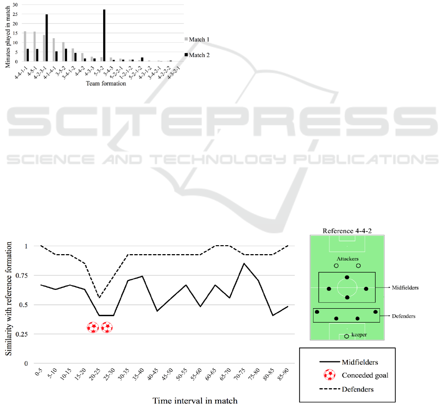
Figure 3: Frequencies of team formations played by an

anonymous team during two matches, ordered according to

the frequencies of match 1.

4.3 Parts of a Team Formation

Going more in detail, it can be interesting to analyse

how different groups of players of a team, e.g.

defenders and midfielders, each stick to their

theoretical formation during a match. Figure 4

displays the compliance of the midfielders and

defenders of an anonymous team with their respective

reference formation throughout one match, with a

temporal resolution of 5 minutes. It can be seen that

the defence much more sticks to its reference

formation throughout the game than the midfield,

which naturally has a more flexible and interchanging

character (Gonçalves et al., 2014). Between minutes

15 and 30 of the match, however, the only period

during which the displayed team conceded (multiple)

goals, both defenders as well as midfielders had the

highest deformations with respect to their reference

formations.

4.4 Analysis of a Team Formation at

Set Pieces

Team formations at set pieces, i.e. corners and free

kicks, are one of the most studied and trained aspects

of team formation in football (Sarmento et al., 2014).

By transforming both the desired as well as the actual

performed formations at set pieces into QTC

matrices, coaches can get an overview of whether and

to what extent the ideal trained-on formation of their

own team was achieved in real matches or get insight

into the tactics and regularly performed team

formations at set pieces of opponent teams.

5 DISCUSSION

In this paper, we presented QTC

, a qualitative

calculus that can be used for team formation analysis

in football. This method can easily be applied to other

sports and incorporates both inter-player coordination

as well as inter-team coordination (Memmert et al,

Figure 4: The similarity of midfielders and defenders of an anonymous team with their reference formation throughout one

game.

Analysing Team Formations in Football with the Static Qualitative Trajectory Calculus

2017). While it has some similarities with already

established methods for team formation analysis (see

Section 2), we are convinced of its added value by its

qualitative character, simplicity and extensibility.

With respect to the qualitative character, we feel

that quantitative methods fail to incorporate the

perception of the players positioning themselves into

the team formation on the field. These perceptions

will more likely be qualitative, e.g. “I am too far

behind the opponent’s midfielder” or “I am standing

too close to my keeper” than quantitative, e.g. “I am

currently 21.45 meters away from my team’s left

winger”. As such we are convinced that qualitative

methods will better grasp the principles players use to

position themselves on the field. Although Ayanegui-

Santiago (2009) already proposed a similar

qualitative method, important differences in this

respect can be noticed. First of all, no distinction

between the studied players is made with QTC

drawing and comparing vectors between all the

players and thus using all spatial information for the

analysis. Secondly, QTC

results are standard

rotation-invariant, although rotation-sensitivity can

be enforced by adding static points (such as the

corners of the football field) to the QTC

description

of a team formation. Thirdly, we believe the QTC

methodology can calculate distance between different

formations more precisely, through the use of

conceptual distances (Van de Weghe and De Maeyer,

2005) between QTC

-characters (instead of the

duality between identity and non-identity between

characters) and the option to extend the number of

QTC

-characters used, conform the extension of

QTC

to QTC

and QTC

(Van de Weghe, De Tré et

al., 2005). Moreover, Ayanegui-Santiago argues that

his work could be enhanced by the conversion of the

numerical orientations between players into

symbolical ones, such as the QTC

-characters.

In Section 4 of this paper, we presented a series of

applications of the QTC

-methodology in football.

The applications, however, are not limited to this list,

as one could for example analyse how a team gets

back into formation in the minutes after conceding a

goal or analyse how substitutions affect the quality of

the team formation, and so on. Furthermore, by

linking the team formation with performance factors

such as scored goals, won matches or ball possession,

coaches could be supported into making better

decisions and ultimately, try to win more games.

We are, however, aware of the lack of concrete

validation of the results in this paper, but would like

to point out the difficulty of validating methods for

(team) formation pattern detection in football due to

the lack of a good ground truth, as argued by

Feuerhake (2016). Furthermore, because of a huge

variety in methodologies, it cannot be assumed that

finding the same results as other established methods

is desirable nor that it should be the goal. As such, we

are convinced that validation should primarily be

done by sports professionals (e.g. coaches).

At the moment, the proposed methodology has

some computational limitations. Permutations

between players, for example, allowing to detect

similarities between formations where two or more

players switch roles, are possible though require high

processing power. As such, when using permutations,

the number of players that can be analysed is limited.

Furthermore, at the moment it is only possible to

compare formations with the same number of players

involved.

6 CONCLUSION

In this paper, we presented QTC

, a novel method for

team formation analysis in football. We explained the

principles of QTC

and illustrated its applicability by

a series of basic football examples. With QTC

, team

formations of both an entire football team as well as

a smaller group of players can be described. Analysis

of these formations can be done for multiple matches,

thereby defining the playing style of a team, or at

critical moments during a game, such as set pieces.

Further research could analyse the impact of static

points or the extension of QTC

to include more

characters on the team formation detection accuracy.

Furthermore, different weights could be allocated to

the vectors between players, according to their

importance on the field.

ACKNOWLEDGEMENTS

The authors would like to thank the Research

Foundation Flanders for funding the research of

Jasper Beernaerts.

REFERENCES

Ahmed, F., Deb, K., Jindal, A. (2013). Multi-objective

optimization and decision making approaches to cricket

team Selection. Applied Soft Computing, 13(1), 402-

414.

Ayanegui-Santiago, H. (2009). Recognizing Team

Formations in Multiagent Systems: Applications in

Robotic Soccer. In Nguyen, N.T., Kowalczyk, R.,

Chen, S.M. (Eds.). Computational Collective

icSPORTS 2018 - 6th International Congress on Sport Sciences Research and Technology Support

Intelligence. Semantic Web, Social Networks and

Multiagent Systems. Lecture notes in computer

science, 5796, 163-173.

Atmosukarto, I., Ghanem, B., Ahuja, S., Muthuswamy, K.,

Ahuja, N. (2013). Automatic recognition of offensive

team formation in American Football plays. 2013 IEEE

Conference on computer vision and pattern

recognition, 991-998.

Barrick, M.R., Stewart, G.L., Neubert, M.J. (1998). Mount

relating member ability and personality to work-team

processes and team effectiveness. Journal of Applied

Psychology, 83, 377-391.

Bialkowski, A., Lucey, P., Carr, P., Yue, Y., Matthews, I.

(2014). “Win at Home and Draw Away”: Automatic

Formation Analysis Highlighting the Differences in

Home and Away Team Behaviors. Disney Research

Boon, B.H., and Sierksma, G. (2003). Team formation:

Matching quality supply and quality demand. European

Journal of Operational Research, 148(2), 277-292.

Bogaert, P., Van de Weghe, N., Cohn., A.G., Witlox, F., De

Maeyer, P. (2007). The Qualitative Trajectory Calculus

on Networks. In Barkowsky, T., Knauff, M., Ligozat,

G., Montello, D. (Eds). Spatial cognition V reasoning,

action, interaction. Lecture notes in computer science,

4387, 20-38. Springer, Berlin, Heidelberg.

Carling, C. (2011). Influence of opposition team formation

on physical and skill-related performance in a

professional soccer team. European Journal of Sport

Science, 11(3), 155-164.

Colleen Stuart, H. (2017). Structural disruption,

experimentation and performance in professional

hockey teams: A network perspective on member

change. Organization Science, 28(2), 283-300.

Dezman, B., Trinic, S., Dizdar, D. (2001). Expert model of

decision making system for efficient orientation of

basketball players to positions and roles in the game -

empirical verification. Collegium Antropologicum,

25(1), 141-152.

D’Orazio, T., and Leo, M. (2010). A review of vision-based

systems for soccer video analysis. Pattern Recognition,

43(8), 2911-2926.

Feuerhake, U. (2016). Recognition of Repetitive movement

patterns-the case of football analysis. International

Journal of Geo-Information, 5(11), 208.

Frencken, W., de Poel, H., Visscher C., Lemmink, K.

(2012). Variability of inter-team distances associated

with match events in elite standard-soccer. Journal of

Sport Science, 30(12), 1207-1213.

Gonalves, B.V., Figueira, B.E., Mas, V., Sampaio, J.

(2014). Effect of player position on movement

behaviour, physical and physiological performances

during an 11-a-side football game. Journal of Sports

Sciences, 32(2), 191-199.

Grunz, A., Memmert, D., Perl, J. (2012). Tactical pattern

recognition in soccer games by means of special self-

organizing maps. Human Movement Science, 31(2),

334-343.

Jäger, M.J., and Schöllhorn, W.I. (2012). Identifying

individuality and variability in team tactics by means of

statistical shape analysis and multilayer perceptrons.

Human Movement Science, 31(2), 303-317.

Kaminka, G.A., Fidanboylu, M., Chang, A., Veloso, M.M.

(2003). Learning the sequential coordinated behavior of

teams from observations. In Kaminka, G.A., Lima,

P.U., Rojas, R. (Eds.). RoboCup 2002: Robotic soccer

world cup VI. Lecture notes in computer science, 111-

125. Springer, Berlin, Heidelberg.

Kuhlmann, G., Stone, P., Lallinger, J. (2005). The UT

Austin villa 2003 champion simulator coach: A

machine learning approach. In Nardi, D., Riedmiller,

M., Sammut, C., Santos-Victor, J. (Eds.). RoboCup

2004: Robot Soccer World Cup VIII. Lecture notes in

computer science, 3276, 636-644. Springer, Berlin,

Heidelberg.

Lemmink, K., and Frencken, W. (2013). Tactical

performance analysis in invasion games: Perspectives

from a dynamical system approach with examples from

soccer. In McGarry, T., O’Dono-ghue, P., Sampaio, J.

(Eds.). Routledge Handbook of Sports Performance

Analysis (pp. 89-100). London: Routledge.

Lucey, P., Bialkowski, A., Carr, P., Morgan, S., Matthews,

I., Sheikh, Y. (2013). Representing and discovering

adversarial team behaviors using player roles. 2013

IEEE Conference on computer vision and pattern

recognition, 2706-2713.

Lucey, P., Bialkowski, A., Carr, P., Yue, Y., Matthews, I.

(2014). “How to get an open shot”: Analyzing team

movement in basketball using tracking data. Disney

research.

Mavridis, N., Belloto, N., Iliopoulos, K., Van de Weghe, N.

(2015). QTC

: extending the qualitative trajectory

calculus to three dimensions. Information Sciences,

322(1), 20-30.

McCulloch, W.S., and Pitts, W. (1943). A logical calculus

of ideas immanent in nervous activity. Bulletin of

Mathematical Biophysics, 5(4), 115-133.

Memmert, D., Lemmink, K.A.P.M., Sampaio, J. (2017).

Current Approaches to Tactical Performance Analysis

in Soccer. Sports Medicine, 47(1), 1-10.

Perin, C., Vuillemot, R., Fekete, J.D. (2013). SoccerStories:

A kick-off for visual soccer analysis. IEEE Trans. Vis.

Comput. Graph, 19(12), 2506-2515.

Rein, R., and Memmert, D. (2016). Big data and tactical

analysis in elite soccer: future challenges and

opportunities for sports science. Springerplus, 5(1),

1410.

Sampaio, J., and Macãs, V. (2012). Measuring tactical

behaviour in football. International Journal of Sports

Medicine, 33(5), 395-401.

Sarmento, H., Pereira, A., Anguera, M., Campanico, J.,

Leitao, J. (2014). The coaching process in football – A

qualitative perspective. Montenegrin Journal of Sports

Science and Medicine, 3(1), 9-16.

Tierney, P.J., Young, A., Clarke, N.D., Duncan, M.J.

(2016). Match play demands of 11 versus 11

professional football using global positioning, system

tracking: Variations across common playing

formations. Human Movement Science, 49(1), 1-8.

Analysing Team Formations in Football with the Static Qualitative Trajectory Calculus

Van de Weghe, N., Cohn. A.G., De Maeyer, P., Witlox, F.

(2005). Representing moving objects in computer-

based expert systems: the overtake event example.

Expert Systems with Applications, 29(4), 977-983.

Van de Weghe, N., and De Maeyer, P. (2005). Conceptual

neighbourhood diagrams for representing moving

objects. Lecture Notes in Computer Science, 3770, 228-

238.

Van de Weghe N., De Tré, G., Kuijpers B., De Maeyer

P. (2005). The double-cross and the generalization

concept as a basis for representing and comparing

shapes of polylines. In Meersman, R., Tari, Z.,

Herrero, P. (Eds.). On the move to meaningful

internet systems 2005: OTM 2005 workshops.

Lecture notes in computer science, 3762, 1087-1096.

Springer, Berlin, Heidelberg.

Visser U., Drücker, C., Hübner, S., Schmidt, E., Weland,

H.G. (2001). Recognizing formations in opponent

teams. In Stone, P., Balch, T., Kraetzschmar, G.

(Eds.). RoboCup 2000: Robot Soccer World Cup IV.

Lecture notes in computer science. Springer, Berlin,

Heidelberg.

icSPORTS 2018 - 6th International Congress on Sport Sciences Research and Technology Support