
Anomaly Detection using System Identification Techniques
Gheorghe Sebestyen and Anca Hangan
Department of Computer Science, Technical University of Cluj-Napoca, Cluj-Napoca, Romania
Keywords: Anomaly Detection, System Identification, Autoregression.
Abstract: As cyber-physical systems are becoming more human independent any anomaly or system failure should be
detected and solved in an autonomous way. In the last decade significant research was performed to find
more intelligent and accurate anomaly detection methods. Most of these methods are analyzing only the
output(s) of a system hoping to find some inconsistencies in the data stream. Our attempt is to consider the
system’s model as well and develop an anomaly detection methodology that tries to identify slight changes
in the behavior of the system, detectable through model changes. The key part of our detection method is
the system identification step through which we compute the system’s model considered as a differential
equation between input and output signals or as an autoregression formula. We demonstrate the feasibility
of the proposed method through a simulated and a real-life example.
1 INTRODUCTION
In cyber-physical systems anomalies may have
various causes like natural ones as environmental
noise, communication errors or device faults as well
as artificial ones caused by malicious attacks (e.g.
virus attacks). In each case an automated method
should discriminate between correct and abnormal
data. In case of computer controlled systems,
incorrect parameter values will produce wrong
control decisions which may bring the physical
system in an unstable, even dangerous state.
Therefore, the measured values should be analyzed,
and outlier values should be eliminated before a
control decision is made.
There are different kinds of anomalies that
should be detected:
• statistically detectable anomalies
• single value outliers (in time series and
spatially distributed data)
• abnormal signal shapes or patterns
• system behavior changes
This article is focused mainly on the detection of
anomalies from the last category where a slight
change in the behavior of a system may be
interpreted as an anomaly. As it will be shown in the
next paragraphs, the problem of anomaly detection
can be solved using system identification techniques.
We measure continuously the input and output of a
given system and compute the coefficients of the
system’s model described as a differential equation
or as an auto-regression. Any significant change in
these coefficients is considered an anomaly. This
detection technique is based on the supposition that
a given physical system is not changing its
mathematical model in time.
This method can detect anomalies that are not so
evident for a human observer. Also, some other kind
of anomaly detection methods based only on the
continuity or statistical parameters of the output
signal may fail to detect changes in the system
model. This method also eliminates some false
anomalies (that may be detected by other methods)
that may occur because of some significant change
in the input signals.
The rest of the paper is organized as follows: the
next section presents some related work in the area
of anomaly detection; section 3 explains the basic
idea behind our method, it gives the mathematical
background and demonstrates the feasibility of the
method through some experiments; the conclusions
of this research are summarized in the last chapter.
2 RELATED WORK
In the last decade, a lot of research was performed
(Barnett et al., 1994) (
Cateni et al, 2008) (Gupta et al,
2014
) in the direction of developing new anomaly
482
Sebestyen, G. and Hangan, A.
Anomaly Detection using System Identification Techniques.
DOI: 10.5220/0006888604820487
In Proceedings of the 15th International Conference on Informatics in Control, Automation and Robotics (ICINCO 2018) - Volume 1, pages 482-487
ISBN: 978-989-758-321-6
Copyright © 2018 by SCITEPRESS – Science and Technology Publications, Lda. All rights reserved

detection methods that assure higher accuracy and
precision in different domains on interest: economy
and business, industry, social sciences, weather and
environmental prediction, etc.
One tendency (
Agrawal et al, 2015
) is to find
general methods that work well on a wide range of
datasets. These methods exploit some inherent
correlations and redundancies present in the
collected data, without analyzing the technical
significance of the different attributes present in the
datasets. For instance, the same clustering method
used for anomaly detection may work well on
financial data as well as on environmental data or
data collected from an industrial process.
The other tendency (
Rassam et al, 2013
) (
Zhang et
al, 2010
) is toward a more specialized approach
where the method and its configuration depend on
the applications’ domain, the type of data (e.g.
statistical data, time series, sensorial data, etc.) and
the kind of anomaly taken into consideration. In
(
Estevez-Tapiador et al, 2014
) the authors present a
taxonomy of anomaly detection methods based on
the above-mentioned criteria.
In principle, any anomaly detection method
(
Chandola et al, 2009
) is built upon some kind of
correlation between the samples of some measured
parameters (or signals); the correlation may be found
in the continuity of a signal (e.g. for time series) or
as a functional correlation between different
parameters (e.g. given by a physical law). An
anomaly is broking these correlation rules, offering
the ground for the automated detection process.
Our proposed method tries to go “behind the
scene” in the sense that it does not look only on the
collected data, it tries to build the model of the
system that generates the data. In our approach any
change in the system model (e.g. behavior) is an
indicator of a possible anomaly. In this sense we
consider that this kind of anomaly detection
technique is a different approach and it may solve
some cases when more traditional methods fail to
detect the anomaly.
3 ANOMALY DETECTION AS A
SYSTEM IDENTIFICATION
PROBLEM
Most of the anomaly detection techniques used for
datasets containing time series try to analyze the
output of a given system in order to identify an
abnormal value or sequence of values. In these
cases, the anomaly detection is based on the
supposition that there is a time correlation between
consecutive samples of the same (process)
parameter. The graphic of the time series should be a
continuous function over time. Any sample that
breaks this correlation is considered an anomaly of
some kind. Sometimes also spatial correlation (e.g.
present in data collected through a distributed sensor
network) or any kind of functional correlation
between multiple parameters may be used for this
purpose.
Unfortunately, in all these cases a significant
change in the evolution of the output signal(s) is
considered an anomaly. But there are justified cases
when the output of a system changes significantly
without it being an anomaly.
For instance, in a temperature regulated room a
door/window is opened, and the temperature is
dropping fast, or in the case of an electric motor the
speed varies significantly if the input voltage of the
load changes. Therefore, in such systems also the
input signal(s) that may produce a change in the
output signal(s) has to be considered, eliminating
those cases when the drastic change of the output
was caused by a justified change in the input.
There are also cases when a system is changing
its behavior without a significant change in the
output signal. As it will be shown in figures 2 and 3
it is hard even for the human eye to determine the
moment when such a change happened. These cases
should also be considered as anomalies in the
behavior of a system.
The goal of our research was to find an anomaly
detection approach that covers both cases: to
eliminate false alarms if a change is caused by
natural causes and to detect slight changes in the
behavior of a system as an indicator for an anomaly.
Figure 1 shows the basic setup of our
experiment. We consider that there is a given system
(a black box) who’s input and output parameters are
measurable. A component, called the estimator, tries
to build the mathematical model of the given system,
based on the measured input and output signals. Any
significant change in the system’s model detected
during the time may be considered as an abnormal
behavior or an anomaly.
Figure 1: The setup scheme.
Anomaly Detection using System Identification Techniques
483

3.1 The Mathematical Approach
In most cases a real (physical) system may be
approximated with a first order or second order
differential equation. This assumption is based on
the fact that most real systems have one or maybe
two dominant time constants that correspond to
some inertial (or energy accumulating) components.
For instance, in electronics an RC filter (resistor
condenser) is described with a first order differential
equation and a circuit with a resistor a condenser and
an inductor as a second order equation (the
condenser and the inductor are the energy
conserving components). In a similar way in
mechanics a suspension system composed of a
spring and a dumper may be modelled with a second
order equation.
A first order differential equation has the
following form:
/ = ∗
() +∗() (1)
Where: y(t) is the output signal and x(t) is the
input signal; A, B are the constants that define the
the system model.
In digital domain, the equation becomes:
(
)
=∗
(
−1
)
+∗
(
)
(2)
Where: y(i), x(i) are the n
th
sample of the output
and input signals; a,b are constants that describe the
first order system.
In a similar way, a second order system is
described in digital domain as:
(
)
=∗
(
−1
)
+∗
(
−2
)
+∗
(
)
(3)
In order to model a given physical system with
an acceptable precision a first or a second order
differential equation is adopted and then the constant
parameters of the equation should be determined.
This process is called system identification. There
are many methods that can be used for this purpose.
For instance, one method works as follows: a step
signal is applied at the input of the system; the
corresponding values measured at the output of the
system will give the integral of the system’s
transformation function. By differentiating the
output signal, we obtain the transformation function
of the system.
In our case the above method cannot be applied
because the identification process should be
continuous, and the input signal is not controlled.
Another issue is the noise which affects the signals
and consequently the correctness of the equation (2).
In the presence of noise equation (2) becomes:
(
)
=∗
(
−1
)
+∗
(
)
+ɛ(n) (4)
Where: ɛ(n) is the error experienced because of
the noise
Therefore, we compute the constants of the first
or second order equations using the measured values
of the output (y) and input (x) signals. In the first
stage we also ignore the error generated by noise.
Its effect will be reduced later using a low-pass-
filter. For instance, in the case of the first order
equation we generate a system of 2 linear algebraic
equations with „a” and „b” as unknown variables.
(
)
=∗
(
−1
)
+∗
(
)
(5)
(
−1
)
=∗
(
−2
)
+∗
(
−1
)
In this way in every sampling moment we obtain
a pair of values a(n) and b(n). In the case of a stable
physical system and without noise the a(n) and the
b(n) values are constant and represent the theoretical
model of the physical system. But because of the
noise the a(n) and b(n) are strongly affected by
noise. Therefore, in order to obtain a “close to
constant” value for “a” and “b” we have to apply a
low pass filter. The length of the median low pass
filter should be adjusted in accordance with the
magnitude of the noise. Another, more accurate
method of determining the „a” and „b” constants
would be to apply a „least square method” that tries
to minimize the sum: Σɛ
2
(n). But in the case of
differential equations this procedure is not a trivial
one. As it will be showed through a practical
example the simpler method proposed here generate
satisfactory results for the anomaly detection
purpose.
The next step in the anomaly detection process is
to follow the evolution of the filtered „a” and „b”
values and determine the moment when the two
parameters change their values in a significant
(detectable) way. The change in the values signifies
a change in the model and consequently a change in
the behavior of the system. This change may be
interpreted as an anomaly.
ICINCO 2018 - 15th International Conference on Informatics in Control, Automation and Robotics
484
3.2 Experimental Demonstration
To show the effectiveness of the proposed anomaly
detection method we present an experimental
simulated case study of a first order physical system.
The experiment considers a RC (resistor condenser)
low pass filter as an example of a first order physical
system. For a more realistic case we consider that
the output signal (the voltage on the condenser) is
affected by a white noise. For a unit step input
signal, the output is given by the equation:
() =∗(1−^(−(/)))+noise (6)
Where: Amp=5V is the amplitude of the input
signal; 1/RC=150s is the time constant of the system
In digital domain the equation of the system
(derived from the analog formula) is:
(
)
=∗
(
−1
)
+∗
(
)
+ (7)
Where: a=0.860707976
b=0.139292024
noise=0.05*(0.5-Random(0÷1))
sample period T=0.002s
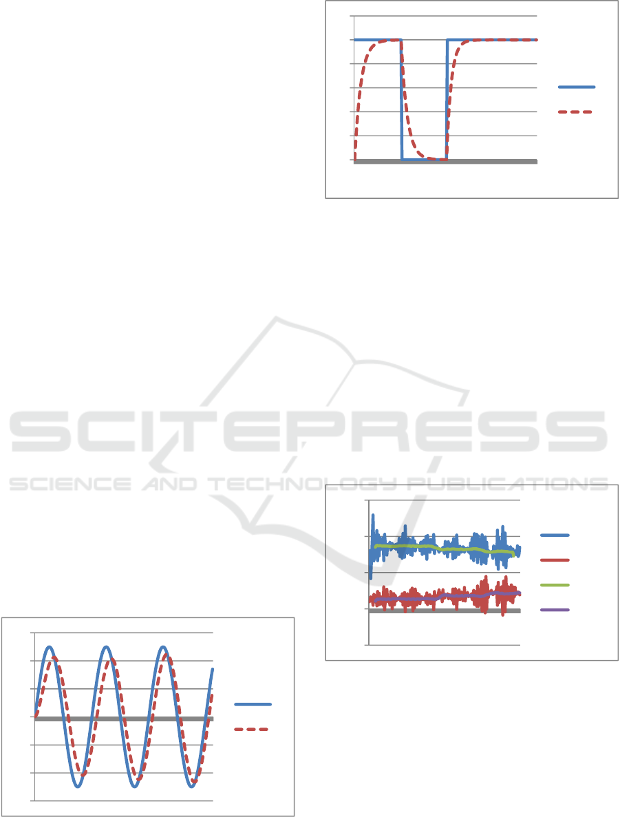
Figures 2 and 3 show the chart of the input and
output signal for a sinus input and a square digital
signal.
What is not so obvious in figures 2 and 3 is the
fact that in both charts the system changed its
behavior two times: once at sample time 90 and
again at sample time 146. First the 1/RC changed
from 150 to 200 and the second time to 250. These
changes are reflected in parameters „a” and „b”.
Figure 2: The input and output signals for an RC circuit
with sinus input.
Figure 3: The input and output signals for an RC circuit
with digital input.
Figure 4 represents the raw values of „a” and „b”
computed using the equation system (5), for each
sampling point. It can be seen that the „constant”
values are strongly affected by the noise. Therefore,
in order to obtain an average value for a and b a
median low-pass-filter is applied. After a number of
experiments the best results were obtained for a
median filter computed on 15 consecutive samples.
Figure 4 shows the filtered values of a, b, (a_LPF
and b_LPF). It can be seen that the filtered values
show a change whenever the system change its
behavior (at approximately 85-95 and 143-150).
These changes may be detected and considered as
anomalies.
Figure 4: Values of a, b and low-pass filterred a_LPF and
b_LPF.
In order to identify the position of the anomaly
(of the change) we applied the following sequence
of operations:
• Modified derivate of the a_LPF and b_LPF with
the formula:
• _
(
)
=_
(
−2
)
+_
(
−
1
)
−_
(
+1
)
+_
(
+2
)
(8)
-6
-4
-2
0
2
4
6
1
21
41
61
81
101
121
141
161
181
x
y
0
1
2
3
4
5
6
1
21
41
61
81
101
121
141
161
181
x
y
-0,5
0
0,5
1
1,5
1
23
45
67
89
111
133
155
177
a
b
a_LPF
b_LPF
Anomaly Detection using System Identification Techniques
485
• _
(
)
=_
(
−2
)
+_
(
−
1
)
−_
(
+1
)
+_
(
+2
)
(9)
• Threshold the a_diff and b_diff with values
between the min and max of the two signals,
obtaining a_thr and b_thr
• Detect the points of change with the condition:
• if(a_thr!=0)AND(b_thr!=0) than detect(n)=1
else detect(n)=0
Figure 5 shows the filtered values (a_LPF,
b_LPF) as well as the result of the detection process.
Figure 5: Detection of the anomaly.
This experiment shows that it is possible to
detect slight changes in the behavior of a system that
may be considered as anomalies. For this purpose,
we measured the input and output signals, computed
the momentary model of the system (coefficients a
and b in the first order differential equations) and
detected a significant change in the computed
model. As the simulated experiment shows, some
parameters of this method (e.g. filter length,
threshold values) must be configured in accordance
with some characteristics of the analyzed system
(e.g. noise level, sampling rate, etc.).
In a very similar way, if the real system has two
dominant time constants a second order differential
equation may be used for the detection (as presented
in equation 3). In this case using a system of 3
equations (similar with 5) we can compute the
coefficients a, b and c. Then any significant change
in these coefficients will indicate a possible
anomaly.
3.3 Variation to the Proposed Detection
Method
In a case when the input signal is not available (not
known), only the output one is measured (e.g.
temperature variations in a given environment, or a
vibration on a mechanical device) the system model
may be approximated as an autoregression model,
using the following equation:
(
)
=
∑
∗(−)
+
(10)
Where:
are the coeficients of the model that
must be computed
N- the order/length of the regression
In case of more complex systems different
variations of autoregression models may be used
such as ARMA, ARIMA or ARMAX. In these cases
the execution time of the detection method may
increase significantly.
In the followings, we present an example of an
anomaly detection on a real case: the problem was to
identify any damages on the bearing of an electric
motor. For this purpose, we measured the vibrations
on the chassis of the motor using an acceleration
sensor. Figure 6 shows the acceleration signal
measured on a motor with damaged bearing. The
high frequency signals on the acceleration indicate
an anomaly in the bearing.
Figure 6: Acceleration signal measured on a faulty motor
bearing.
In this case we used the following equation:
(
)
=
∗
(
−1
)
+
∗
(
−2
)
+
(11)
Figure 7: The variation of the c1 coefficient.
We observed that the coefficient that best
reflects the anomaly is in this case
1
. Figure 7
shows the variation of coefficient c1 over the
original signal.
0
0,5
1
1,5
1
30
59
88
117
146
175
a_LPF
b_LPF
detectio
n
ICINCO 2018 - 15th International Conference on Informatics in Control, Automation and Robotics
486
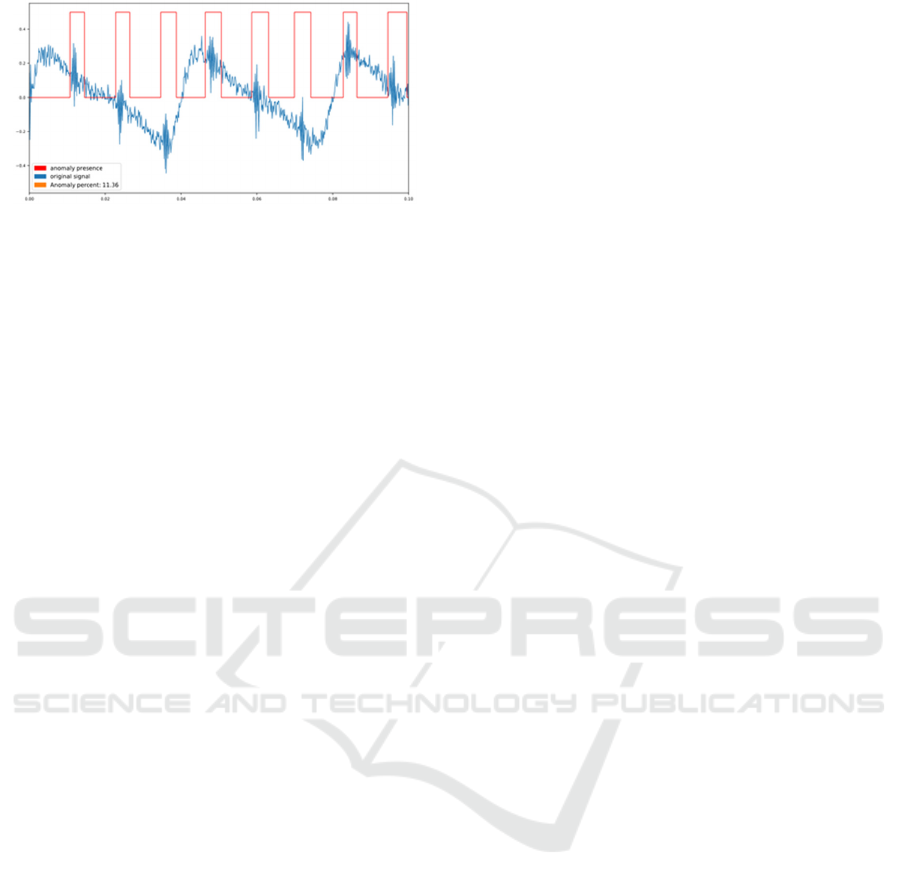
Figure 8: Labeled anomaly regions.
The next step was to apply a thresholding
method in order to identify regions with faulty
signals. The value of the threshold is determined in
this case automatically from the histogram of the C1
values: the threshold value is the lowest point of a
„valley” that separate the normal and abnormal c1
values. Figure 8 shows the final result with the
labeled values.
4 CONCLUSIONS
This paper showed that anomaly detection methods
may be derived from a system identification method.
The first example considered a system that may be
described with a first order differential equation. The
coefficients a and b of the discrete equation show
variations that can be exploited for anomaly
detection. The second example considered a system
where the input signal is not known. In this case an
autoregression model was computed. Again, one of
the coefficients of the discrete formula could be used
for anomaly detection.
In both cases the actual sequence of processing
steps needed for an accurate detection had to be
adjusted with the specific characteristics of the
analyzed system. So, from this point of view a
single method cannot be generally applied to any
real-life problems. But, with some adjustments the
proposed method may solve a wider range of
applications.
As it was demonstrated, the proposed anomaly
detection method can detect slight changes in the
behavior of a given system, that can be interpreted
as anomalies and which may not be detected by
more traditional methods or even by a human
observer. The proposed method also eliminate false
anomaly alerts which are caused by significant
changes in the input signal that affect also the
output; usually other anomaly methods ignore the
input signal and its effect on the output signal.
The proposed method is rather simple and may
be implemented on embedded devices with limited
computing or storage capabilities, such as
microcontrollers or DSPs. It is also recommended
for on-line anomaly detection.
As future work, we intend to apply pattern
recognition and classification methods (e.g. neural
networks and SVM) on the graph of the computed
model coefficients in order to discriminate between
normal and abnormal system behaviors.
ACKNOWLEDGMENT
The results presented in this paper were obtained
with the support of the Technical University of Cluj-
Napoca through the research Contract no.
1995/12.07.2017, Internal Competition CICDI-2017.
REFERENCES
Barnett, V. and Lewis, T., 1994 Outliers in Statistical
Data, New York: John Wiley Sons.
Chandola, V., Banerjee, A., Kumar, V., 2009. Anomaly
Detection: A Survey ACM Computing Surveys 41, 3.
Estevez-Tapiador, J. M., Garcia-Teodoro, P., Diaz-
Verdejo, J. E., 2014 Anomaly detection methods in
wired networks: a survey and taxonomy, Computer
Communications, volume 27
Rassam, M. A.; Zainal, A.; Maarof, M. A., 2013
Advancements of Data Anomaly Detection Research
in Wireless Sensor Networks: A Survey and Open
Issues. Sensors, 13, 10087-10122.
Agrawal, S., Agrawal, J., 2015 Survey on Anomaly
Detection using Data Mining Techniques, 19th
International Conference on Knowledge Based and
Intelligent Information and Engineering Systems, ed.
Elsevier, Procedia Computer Science 60, 708 713
Gupta, M., Gao, J., Aggarwal, C. C., Han, J., 2014 Outlier
Detection for Temporal Data: A Survey, IEEE
Transactions On Knowledge And Data Engineering,
vol. 25, no. 1
Cateni, S., Colla, V. and Vannucci, M., 2008 Outlier
Detection Methods for Industrial Applications, chapter
in book “Advances in Robotics, Automation and
Control”, book edited by Jesus Aramburo and Antonio
Ramirez Trevino, ISBN 978-953-7619-16-9
Zhang Y., Meratnia N., and Havinga P., 2010 Outlier
Detection Techniques for Wireless Sensor Networks:
A Survey, IEEE Communications Surveys and
Tutorials, vol. 12, no. 2.
Anomaly Detection using System Identification Techniques
487
