An Approach for Adaptive Parameter Setting

in Manufacturing Processes

Sonja Strasser, Shailesh Tripathi and Richard Kerschbaumer

Production and Operations Management, University of Applied Sciences Upper Austria,

Wehrgrabengasse 1-3, Steyr, Austria

Keywords: Process Parameter Setting, Manufacturing, Model Selection, Regression Analysis, Machine Learning.

Abstract: In traditional manufacturing processes the selection of appropriate process parameters can be a difficult task

which relies on rule-based schemes, expertise and domain knowledge of highly skilled workers. Usually the

parameter settings remain the same for one production lot, if an acceptable quality is reached. However, each

part processed has its own history and slightly different properties. Individual parameter settings for each part

can further increase the quality and reduce scrap. Machine learning methods offer the opportunity to generate

models based on experimental data, which predict optimal parameters depending on the state of the produced

part and its manufacturing conditions. In this paper, we present an approach for selecting variables, building

and evaluating models for adaptive parameter settings in manufacturing processes and the application to a

real-world use case.

1 INTRODUCTION

Product and process quality is playing an increasingly

important role in the competitive success of

manufacturing companies (Robinson and Malhotra

2005). As a consequence, this trend forces

manufacturing companies to further improve their

production (Wuest et al., 2014).

In general, quality is defined as the degree to

which a commodity meets the requirements of the

customer (DIN EN ISO 9001:2015). In this context,

customers are not only the users of final products;

they can also be other companies in a supply chain

network. When a company is a supplier of

components, which serve as assembly parts in a final

product, then important quality requirements are

dimensions of parts, which have to be within

predefined tolerances. There exist International

Tolerance Grades of industrial processes, which

identify what tolerances a given process can produce

for a given dimension (ISO 286-1:2010). If an

industrial process is more precise, less scrap is

produced or even a higher tolerance class can be

achieved and the produced components can generate

more profit for the company.

The appropriate and prompt selection of process

parameters in manufacturing processes plays a

significant role to ensure the quality of the product, to

reduce the machining cost and to increase the

productivity of the process (Pawar and Rao, 2013). In

practice, the adjustment of process parameters to get

dimensions of a produced part in predefined

tolerances can be a difficult task. Traditional control

systems rely on rule-based schemes, expertise and

domain knowledge of highly skilled workers or on

trial and error. Furthermore, modern manufacturing

processes are becoming more and more complex and

modelling every aspect of a process in a rule- and

expert-based system is getting challenging or even

impossible.

The phase of parameter adjustment consumes

precious production time where scrap parts are

processed. Once an acceptable setting of parameters

is obtained, it is common to remain it unchanged for

the whole production lot. However, each part

processed has its own history and slightly different

properties. Individual parameter settings for each part

can further increase the quality and reduce scrap.

Machine learning (ML) methods offer the

opportunity to generate models based on

experimental data, which automatically predict

optimal parameters depending on the state of the

produced part and its manufacturing conditions.

This paper contributes to the application of ML

methods for parameter setting in manufacturing

processes and addresses the following research ques-

Strasser, S., Tripathi, S. and Kerschbaumer, R.

An Approach for Adaptive Parameter Setting in Manufacturing Processes.

DOI: 10.5220/0006894600240032

In Proceedings of the 7th International Conference on Data Science, Technology and Applications (DATA 2018), pages 24-32

ISBN: 978-989-758-318-6

tions:

- How can ML methods be integrated in a

framework for adaptive parameter setting?

- Which ML methods are suitable in models for

adaptive parameters settings?

- Which accuracy can be reached when predicting

quality measures and is this accuracy sufficient

for practical applications?

We provide the related work to this topic in Section 2

and present the methodology of the developed

approach in Section 3. Afterwards, we apply and

evaluate our approach in a use case based on real-

world manufacturing data in Section 4. Concluding

remarks follow in the final Section 5.

2 RELATED WORK

There exist literature of parameter optimization and

parameter setting for different kinds of manufacturing

processes.

For the injection moulding process there are

different approaches. A common design method to

reduce the amount of simulation runs and to consider

interaction effects of parameters is the Taguchi

method (Oliaei et al., 2016; Tian et al., 2017). It is

used to find a better initial point for the optimization

and to reduce time for solving the problem. For the

optimisation of a multi-objective problem a

combination of Response Surface Methodology

(RSM) and non-dominated sorting genetic algorithm

II (NSGA II) is used (Park and Nguyen, 2014; Tian et

al., 2017). The function generated out of the RSM is

optimized with the NSGA II. As initial values for the

first iteration of the genetic algorithm it is possible to

use results from the Taguchi method or to generate

random values within a set range. Oliaei et al., (2016)

used an Artificial Neural Networks (ANN) with the

learning algorithm of back-propagation to optimize

the quality. In their work, they compared the results

of the Taguchi method with the results of the ANN.

In both methods the same sample set was used. The

results show that there is a slight difference between

them.

In Additive Manufacturing unsuitable process

parameters influence the quality of 3D printed parts

adversely. There exist various approaches to use

Machine Learning to choose optimal process

parameters for different technologies in 3D printing

(Fused Deposition Modeling, Selective Laser Melting

or Sintering). The most popular method used is

Artificial Neural Networks (ANN) (Collins et al.,

(2014), Ding et al., (2016)) which performs good due

to the provided flexibility. Although comparisons

show that in some cases regression is only slightly

worse (Xiong et al., (2014), Mohamed et al., 2016).

Cook et al., (2000) develop an ANN to model the

relationship between process operating parameters

and a critical strength parameter in a particleboard

manufacturing process. Then a genetic algorithm is

applied to determine the process parameter values,

which result in desired levels of the strength

parameter.

Park and Kim (1998) present a review on artificial

intelligence approach which attempt to automatically

adapt and optimize the CNC machining parameters

based on sensor information in real time. Again ANN

is the dominating method in this field of application.

Venkata Rao and Kalyankar (2013) present an

approach for process parameter optimization in a

multi-pass turning operation. They developed a

teaching-learning-based optimization algorithm,

which outperforms other optimization methods in

their multi-objective and single-objective examples.

It is stated that this algorithm can be easily modified

for parameter optimization of other manufacturing

processes, such as casting, forming and welding.

An approach for estimating control parameters of

a plasma nitriding process is presented in Kommenda

et al., (2015). They solve inverse optimization

problems to find good combinations of parameters

such that desired product qualities can be fulfilled

simultaneously.

As already slight variations of the product state

during production can lead to costly and time-

consuming rework or even scrap, Wuest et al., (2014)

suggest an approach based on recording of the

individual product’s state along the entire production

process. Whereas condition monitoring is mostly

focused on a single manufacturing process,

monitoring of the whole manufacturing programme

has to be further investigated (Choudhary et al.,

2009). Wuest et al., (2014) suggest a combination of

cluster analysis and support vector machines (SVM)

to achieve the goal of improved quality monitoring.

They provide a theoretical example to illustrate the

potential of the approach, but the application to a real-

life manufacturing process is missing.

This paper applies the concept of tracking the

individual product state to predict quality relevant

requirements of finished manufactured parts. As the

considered target variables are numeric (e.g.

dimensions of the part), instead of classification (e.g.

good and bad parts), methods for regression are

chosen. Furthermore, the developed approach is

evaluated on data from a real-life industrial

environment.

An Approach for Adaptive Parameter Setting in Manufacturing Processes

3 METHODOLOGY

In this section, an approach for the setting of process

parameters of a manufacturing process is developed.

The setting of the process parameter is adaptive for

each produced part depending on its properties and

previous manufacturing conditions. First, the

collection of the necessary process and product data

is presented. Then the basic concept of the parameter

setting is introduced. Based on this concept the next

steps are data pre-processing, the selection of a

suitable machine learning model and its evaluation

based on different criteria.

3.1 Data Collection

We consider a multi-stage manufacturing process,

consisting of N consecutive steps (Figure 1). In each

step a physical transformation of the product is

performed, so that, starting from the raw material in

step 1, the final product is finished in step N. The

approach, which is developed in this section, refers to

parts of one specific product type. If there are

multiple product types in the manufacturing system,

it is possible to apply this approach to each type

separately.

The basic idea is to record all relevant product and

process variables of each manufactured part. Due to

variations in material properties and manufacturing

conditions (e.g. machine and tool conditions,

environmental conditions, influence of human

workers) each part will be characterised by individual

values of the variables, which describe the life cycle

of the part during the manufacturing process. This

concept is introduced by Wuest et al., (2011) as

product state based view.

In our approach, it is important to distinguish

between independent and dependent variables. Some

of the product and process variables, like the type of

raw material or the adjustment of process parameters,

can be manually selected and are not influenced by

other recorded variables. Other variables, like quality

relevant properties of the part, depend on the values

of multiple variables, although the precise

relationships are not known in practice.

Figure 1: Product and Process Variables.

3.2 Basic Concept

The final objective is to determine appropriate,

adaptive parameter settings of the last production step

for a specific part based on its manufacturing life

cycle to fulfil the quality requirements. The selection

of multiple process parameters is likely to deliver a

manifold of solutions whereas the fulfilment of

multiple quality requirements won’t be feasible in

general. Therefore, we restrict our approach to the

determination of one process parameter of the last

production step (u), in order to fulfil a single relevant

quality requirement (z). The considered process

parameter belongs to the independent process

variables of step N and the quality requirement is part

of the dependent product variables of step N. In our

approach, we take only numeric quality measures into

account, like critical dimensions or the weight of the

part.

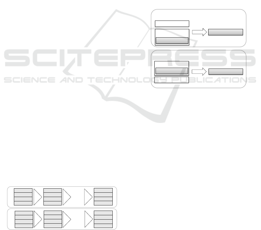
Figure 2: Basic Concept.

To achieve this goal, we suggest a two-step

approach (see Figure 2). First, we model the

relationship between the quality measure and relevant

product and process variables, including the selected

process parameter, by a function f.

( , , )

ij ij

z f x y u

(1)

This function enables the prediction of the relevant

quality measure (

) based on the life cycle of an

individual part. Then we calculate, if possible, the

inverse function of f. This inverse function



enables us to set a predefined optimal value for the

quality measure and to estimate the necessary process

parameter (

) under consideration of the actual

product and process variables of a specific part.

( , , )

ij ij

u f x y z





(2)

If f is no bijective function, Eq. (1) has to be solved

PROCESS

PRODUCT

STEP 1

STEP 2 STEP N

........

Proc

. Var. y

Proc

. Var. y

.....

Proc

. Var. y

Prod

. Var. x

Prod

. Var. x

.....

Prod

. Var. x

Proc

. Var. y

Proc

. Var. y

.....

Proc

. Var. y

Prod

. Var. x

Prod

. Var. x

.....

Prod

. Var. x

Prod

. Var. x

Prod

. Var. x

.....

Prod

. Var. x

Proc

. Var. y

Proc

. Var. y

.....

Proc

. Var. y

MODELING RELATIONSHIP

Product Variables

Process Variables

Process Parameter

-1

PARAMETER SETTING

Product Variables

Process Variables

Process Parameter

Quality Measure

DATA 2018 - 7th International Conference on Data Science, Technology and Applications

implicitly, for example by using Newton’s method.

However, in this case, multiple solutions can exist.

3.3 Data Pre-processing

There are some data pre-processing needed, in order

that we are able to apply regression models in the first

step of our approach. If there are nominal variables in

the set of the recorded product and process variables,

they have to be replaced by binary attributes (dummy

coding). A nominal variable with m levels has to be

transformed in m-1 dummy variables with 0 and 1 as

possible values.

The second point, which has to be checked, is the

collinearity of attributes, since it reduces the accuracy

of the regression model. It is likely that some of the

recorded product and process variables are correlated.

For example, if the height of the part is measured after

each process step, i.e. N times, then these N variables

are presumably more or less correlated. Here not only

correlation between two attributes has to be

considered, also multicollinearity has to be detected.

A way to assess multicollinearity is to compute

variance inflation factors (VIF). The smallest possible

value for VIF is 1, which indicates no collinearity.

Attributes with VIF values that exceed 5 or 10 should

be dropped from the regression analysis (James et al.,

2013).

In some cases, it can be useful to create new

features based on the recorded process and product

variables to increase the accuracy of the applied

machine learning model. Using domain knowledge of

experienced workers of the considered manufacturing

process can help in feature engineering as well as in

the selection of relevant variables.

3.4 Model and Variable Selection

For modelling the relationship between product and

process variables and the quality measure, regression

models and artificial neural networks (ANN) are

applied.

ANN are a flexible and widely spread method for

modelling complex relationships (Widrow et al.,

1994). A multi-layered architecture is built up from

one or more hidden layers placed between an input

and an output layer. Each layer consists of several

highly interconnected processing units, called

neurons, which sum weighted inputs and apply an

activation function for generating the output. The

weights are determined by training the neural network

with the goal to minimize the error between the actual

and predicted output values. Then a separate test set

of data is used to estimate the network’s performance

on new data. After all, the neural network serves as a

function that maps input values (product and process

variables) to output values (quality measures).

Although ANN deliver good models for prediction,

regression models are more transparent and easier to

interpret when applying them in the practice of

manufacturing companies.

When we choose a regression model, we first have

to answer the question, which variables from the set

of the recorded product and process variables of the

whole manufacturing process have the biggest

influence on the quality measure and therefore should

be used for modelling. From the point of view of the

practitioners in the companies, it is desirable to get a

model with a good accuracy, which only depends on

a few variables. This configuration would reduce the

cost and time for measuring and recording a huge

amount of data from the production process.

However, using too few variables will lead to bias and

the inclusion of too many of them is likely to cause

overfitting. A variety of methods for selecting

variables is available (Miller, 2002; James et al.,

2013), such as

 Best subset selection

 Forward selection

 Backward elimination

Best subset selection fits a model to each combination

of possible numbers of prediction variables. If there

are p prediction variables, then

models are trained

and the best of them is selected. Because of the

computational effort, the application is only possible,

if p is not too high. Otherwise, stepwise methods, like

forward selection and backward elimination, are

alternatives, which only explore a restricted set of

combinations. Forward selection starts with the best

model containing only one variable and increases the

number of variables in each step by one. Conversely,

backward selection starts with all possible prediction

variables and reduces the number in each step by one.

Regardless of the applied method for variable

selection, performance measures for the comparison

of different models are necessary in order to pick out

the best model (Murtaugh, 2010). Different

techniques for model evaluation are introduced in the

next subsection 3.4.

If linear regression is not adequate to generate

models with good performance, the linearity

assumption can be relaxed by introducing polynomial

terms or generalized additive models. The selection

of the applied function types can be motivated by

known physical relationships of product and process

variables.

An Approach for Adaptive Parameter Setting in Manufacturing Processes

3.5 Model Evaluation and Parameter

Setting

Different models based on different sets of prediction

variables have to be compared in order to select the

best one. Residual Sum of Squares (RSS) and R² are

not suitable measures because they are based on the

training data and are getting better, when the number

of prediction variables increases. For model selection,

the test error has to be estimated directly (e.g. by

cross-validation) or indirectly (by adjusting the

training error to account for the bias due to

overfitting). In the first case, mean squared error

(MSE) or root mean squared error (RMSE) can be

applied. In the second case, the following criteria can

be used: Akaike information criterion (AIC),

Bayesian information criterion (BIC), C

value and

Adjusted R² (James et al., 2013).

One of these criteria or the cross-validation error

can be applied for model selection in order to get a

linear regression model f based on a selected set of

process and product variables or a neural net with an

optimal number of neurons in the hidden layer. In

variable selection, it must be observed that the

process parameter u, which has to be adjusted for

each individual part, is included in the set of selected

prediction variables. By calculating the inverse

function



of the linear function and inserting the

optimal value of the quality measure z and the

individual product and process variables of a part, an

estimation

for the parameter setting is yield.

4 CASE STUDY

In this section, the developed approach is applied to a

real-world production process in metal processing

industry, which consists of three production steps.

The whole workflow for parameter setting was

implemented in R, an open-source software for

statistical computing. In the next subsection, we

describe the data, which was recorded in a

manufacturing company. There exist two relevant

quality measures of the finished part, so the approach

is applied twice and the results are reported in the

following sections.

4.1 Experimental Data

In an experiment, the data of 200 produced parts and

the associated process data were recorded. Together

with experts of the involved production processes,

relevant variables have been selected. Table 1 shows

the number of the analysed variables of each

production step. According to Figure 1, the following

notation is used:



: j-th product variables of step i



: j-th process variable of step i

Product variables include, for instance, the

dimensions of the part after each process step and its

weight. Important process variables are temperatures,

pressures and forces.

Both product variables of step 3 are important

quality measures, namely the height (

1 31

zx

) and

the diameter (

2 32

zx

) of the part. One of the process

variables of step 3 (

uy

) is the process parameter

which should be determined individually for each part

produced. With the exception of

, all product and

process variables are numeric. Since

is a nominal

attribute with 5 different levels, it is replaced by four

binary attributes (

231 232 233 234

, , ,y y y y

), such as

proposed in section 3.2.

Table 1: Number of Product and Process Variables.

4.2 Results for Quality Measure 1

Here the first quality measure, the height of the

finished part

1 31

zx

, is used as response variable in

a linear regression model. In this model, the second

quality measure

has to be excluded from the

analysis, because it is not available in advance when

using the regression model for prediction.

The calculation of VIF, using the R package “car”,

reveals that there is just one process variable with a

VIF higher than 10 (

 

VIF 12.16x 

). After the

elimination of this variable, the VIF are calculated

again with the result that the maximum value is 7.56.

So this reduced data set is used for building the

regression model.

Since the number of variables is relatively small

in our application, best subset selection can be applied

for model selection. For this purpose we use the

“regsubsets” function from the R-package “leaps”.

Representative for the evaluation of the criteria

mentioned in Section 3.4, Figure 3 displays the results

of adjusted R².

Variables

Step 1 Step 2 Step 3 Total

Product Variables

Process

Variables

Total

DATA 2018 - 7th International Conference on Data Science, Technology and Applications

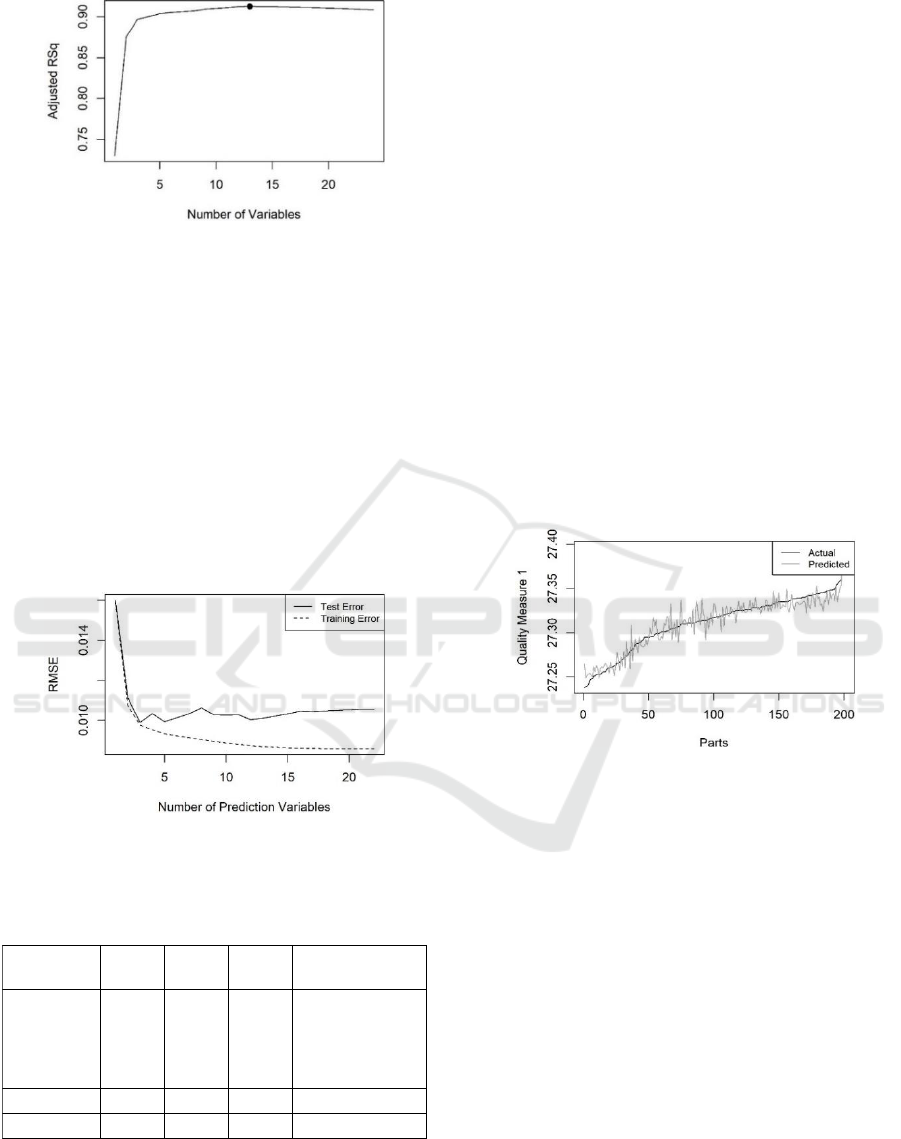
Figure 3: Adjusted R squared for Linear Regression

Models.

Although the optimal number of variables varies

from 5 to 13, all criteria reach good values with just a

view number of variables. A closer look at adjusted

R² reveals, that already 3 variables achieve a result

that is close to the optimal value.

Additionally, 10-fold cross-validation was

applied to best subset selection, to get a better

estimation of the test error. Figure 4 displays the

comparison of test and training error depending on

the number of prediction variables. This evaluation

indicates also that 3 to 5 variables are a good choice

for the regression model.

Figure 4: Cross-validation of Linear Regression Models for

Quality Measure 1.

Table 2: Comparison of Linear Regression Models for

Quality Measure 1.

Now the linear regression model is trained on the

whole dataset in order to obtain models with 3, 4, 5

and 8 variables. Table 2 compares the values of

adjusted R² and RMSE for these models and reveals

that all of these models lead to similar good results.

In all of the models the process parameter

, the

product variable

and the dummy coded process

variable

231

are selected.

The formula obtained by linear regression for

estimating quality measure 1 as a function of three

prediction variables is:

 

1 31 21 231

21 231

18.477 0.772 0.289 0.012

z x f u x y

x u y

  

   

(3)

Therefore, we can see that the quality measure

increases when

increases and it decreases, when

the process parameter

increases or the binary

variable

231

has the value 1. The experts of the

manufacturing company confirm these relationships,

although for them it was surprising, that a linear

function with only three variables can provide good

estimates for this quality measure. Figure 5 provides

a graphical comparison of actual and predicted values

of the quality measure.

Figure 5: Actual vs. Predicted Values for Quality Measure

1 using Linear Regression.

In order to be able to better assess the results, it is

important to know that the optimal value for the

quality measure is 27.29 and the accepted tolerance is

0.06. Partly, there exist quite large deviations from

the optimal value, which is the consequence of the

rather large variations of possible parameters (in

comparison to serial operation) in the experiment to

get better insights in the relationships of product and

process variables. However, the deviation of

predicted values to actual values is less than the

tolerance.

Calculating the inverse function of f and inserting

the optimal value for the quality measure in Eq. (3)

yields a function for the process parameter:

21 231

27.29

30.495 2.671 0.042

u x y



   

(4)

This equation can be applied to estimate the process

Number

Variables

3 4 5 8

Variables

231

, y

232

, y

233

, y

234

Adjusted

R² 0.897 0.900 0.904 0.907

RMSE

0.00977

0.00958

0.00939

0.00914

An Approach for Adaptive Parameter Setting in Manufacturing Processes

parameter u of step 3 individually for each part, just

by inserting one product variable and one process

variable of step 2.

For the purpose of benchmarking the results from

linear regression models, we also apply ANN for

regression. This is done by the “neuralnet” function

of the “neuralnet” package in R. We select a neural

net with one hidden layer and apply 10-fold cross-

validation to get the optimal number of neurons in this

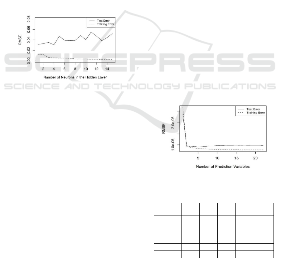
hidden layer, using a range from 1 to 15. Figure 6

shows the training and test error as a function of the

number of neurons in the hidden layer, with a

minimum test error for four neurons. The training

errors of neural networks are comparable to the

training errors for linear regression models (see

Figure 4), but the test errors for ANN are significantly

higher. One reason for this could be the small number

of datasets for training the neural net. So already

models with three neurons tend to overfit the training

data and lead to relatively high test errors.

Figure 6: Cross-validation of Neural Networks for Quality

Measure 1.

When the neural net with four neurons in the

hidden layer is trained on the whole dataset, the

following performance is obtained:

² 0.967

0.00517

Adjusted R

RMSE



(5)

These values outperform the good results from linear

regression (see Table 2), however it is important to

note that the performance of the neural net on new

data is considerably worse than for linear regression.

Further drawbacks of neural nets in this application is

the number of variables applied (and the associated

measuring effort) and the impossibility to calculate an

inverse function, which is required for Eq. (2).

4.3 Results for Quality Measure 2

Now the same approach is applied to quality measure

2, the diameter of the finished part. Again the reduced

dataset without the product variable

, due to its

multicollinearity detected by calculating VIF, is used.

Only the response variable

is replaced by

However, the first results are not very promising.

Training a linear regression model on the whole

dataset using all variables delivers adjusted R² of only

0.07. A neural net can increase this value at 0.2, which

is also too less for practical applications. At this point,

feature engineering is necessary to improve the

results. A detailed analysis revealed that it is

favourable to replace the diameter in step 3 as

response variable by the change of the diameter from

step 2 to step 3:

2 2 32 22

z d x x  

. Additionally we

introduced the change of the diameter from step 1 to

step 2 as a new feature

1 22 12

d x x

and excluded

the diameter

from the analysis for the sake of

collinearity.

First, best subset selection for linear regression

models in combination with a 10-fold cross-

validation is applied for model selection (Figure 7).

Also for the change of the diameter, a small number

of variables (2 – 5) is sufficient for a good predictive

model. In Table 3 linear models, which are trained on

the full data set with 2, 3, 4 and 5 variables, are

compared. Adjusted R² is nearly equally excellent for

all these models. For parameter setting, the first

model is not suitable, because the process parameter

u is not used for prediction. Selection of three

variables for prediction of the change in diameter

yields the function

 

2 2 12 1

12 1

45.982 1.054 0.009 0.972

z d f u x d

x u d

  

   

(6)

Figure 7: Cross-validation of Linear Regression Models for

Change in Diameter.

Table 3: Comparison of Models for Change in Diameter.

Number

Variables

2 3 4 5

Variables

Adjusted

R² 0.974 0.975 0.976 0.976

RMSE

0.00304

0.00296

0.00294

0.00290

DATA 2018 - 7th International Conference on Data Science, Technology and Applications

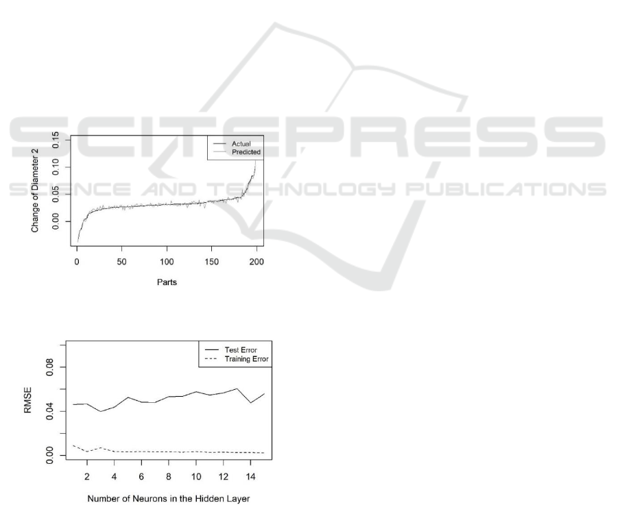
Figure 8 shows the comparison of actual and

predicted values for the change in diameter. The

accepted tolerance for this diameter is 0.012 and the

optimal value is 44.043, which can be applied for

calculating estimates of the necessary process

parameter for individual parts:

22 2

12 1 22

44.043

215.44 117.11 108 111.11

u x d x

  

    

(7)

Also for this quality measure we train a neural net

with one hidden layer and select the optimal number

of neurons with a 10-fold cross-validation. Here three

neurons lead to the minimum test error in the studied

range from 1 to 15 (see Figur). The performance of

the neural net, trained on the whole data set, can be

assessed by the following measures:

² 0.976

0.00275

Adjusted R

RMSE



(8)

Adjusted R² is roughly equal than the value for linear

regression models and RMSE is slightly better (see

Table 3). Taking into account the higher test error for

ANN (Figur) and the drawbacks already discussed for

quality measure 1, also for quality measure 2 the

linear regression model should be preferred.

Figure 8: Actual vs. Predicted Values for Change in

Diameter.

Figure 9: Cross-validation of Neural Networks for Change

in Diameter.

5 CONCLUSIONS

In this article, we present an approach for parameter

setting in manufacturing processes. The parameter

adjustment is adaptive to the properties and history of

each individual part. In the first step the relationship

between multiple input variables and a relevant

quality measure is investigated. Then this relationship

is used to calculate estimates for a specific process

parameter in order to get optimal quality measures.

The results of the case study, based on real-world

manufacturing data, show that even simple linear

regression models with a few product and process

variables provide good estimates for quality measures

and can be applied for parameter setting. We also

train neural nets to get a benchmark for the linear

regression models. The results reveal that neural nets

outperform linear regression on the training data, but

application on the test data shows a significantly

higher test error. Recording more data for training and

testing could be favourable for neural networks.

In further research, we want to extend the

approach to multiple quality measures, which are

weighted in an objective function. In order to

investigate the scalability of the presented approach,

we plan to apply it in a long-term study on a larger

data set of the considered real-world use case. To

evaluate the generality of our approach we intend the

application in other manufacturing processes as well.

ACKNOWLEDGEMENTS

This paper was funded through the projects ADAPT

and BAPDEC by the Government of Upper Austria

in their programme “Innovative Upper Austria 2020”.

REFERENCES

Barz, Christiane, and Rainer Kolisch. 2014. “Hierarchical

Multi-skill Resource Assignment in the

Telecommunications Industry.” Production and

Operations Management 23 (3): 489–503.

doi:10.1111/poms.12053.

Choudhary, A. K., J. A. Harding, and M. K. Tiwari. 2009.

“Data mining in manufacturing: A review based on the

kind of knowledge.” Journal of Intelligent

Manufacturing 20 (5): 501–21. doi:10.1007/s10845-

008-0145-x.

Collins, P. C., C. V. Haden, I. Ghamarian, B. J. Hayes, T.

Ales, G. Penso, V. Dixit, and G. Harlow. 2014.

“Progress Toward an Integration of Process–Structure–

Property–Performance Models for “Three-Dimensional

An Approach for Adaptive Parameter Setting in Manufacturing Processes

(3-D) Printing” of Titanium Alloys.” JOM 66 (7):

1299–1309. doi:10.1007/s11837-014-1007-y.

Cook, D. F., C. T. Ragsdale, and R. L. Major. 2000.

“Combining a neural network with a genetic algorithm

for process parameter optimization.” Engineering

Applications of Artificial Intelligence 13 (4): 391–96.

doi:10.1016/S0952-1976(00)00021-X.

Quality management systems - Fundamentals and

vocabulary (ISO 9000:2015). DIN EN ISO 9001:2015.

2015.

Ding, Donghong, Chen Shen, Zengxi Pan, Dominic Cuiuri,

Huijun Li, Nathan Larkin, and Stephen van Duin. 2016.

“Towards an automated robotic arc-welding-based

additive manufacturing system from CAD to finished

part.” Computer-Aided Design 73: 66–75.

Geometrical product specifications (GPS) — ISO code

system for tolerances on linear sizes. ISO 286-1:2010.

2010.

James, Gareth, Daniela Witten, Trevor Hastie, and Robert

Tibshirani. 2013. An introduction to statistical

learning: With applications in R. Springer texts in

statistics 103. New York: Springer.

Kommenda, M., B. Burlacu, R. Holecek, A. Gebeshuber,

and M. Affenzeller. 2015. “Heat treatment process

parameter estimation using heuristic optimization

algorithms.” In Proceedings of the European Modeling

and Simulation Symposium, edited by M Affenzeller,

Bruzzone, Jimenez, Longo, Merkuryev, and Zhang,

222–27.

Miller, Alan J. 2002. Subset selection in regression. 2nd ed.

Monographs on statistics and applied probability 95.

Boca Raton: Chapman & Hall/CRC.

Mohamed, Omar A., Syed H. Masood, and Jahar L.

Bhowmik. 2016. “Investigation of dynamic elastic

deformation of parts processed by fused deposition

modeling additive manufacturing.” Advances in

Production Engineering & Management 11 (3): 227–

38. doi:10.14743/apem2016.3.223.

Murtaugh, Paul A. 2010. “Methods of variable selection in

regression modeling.” Communications in Statistics -

Simulation and Computation 27 (3): 711–34.

doi:10.1080/03610919808813505.

Oliaei, Erfan, Behzad S. Heidari, Seyed M. Davachi,

Mozhgan Bahrami, Saeed Davoodi, Iman Hejazi, and

Javad Seyfi. 2016. “Warpage and Shrinkage

Optimization of Injection-Molded Plastic Spoon Parts

for Biodegradable Polymers Using Taguchi, ANOVA

and Artificial Neural Network Methods.” Journal of

Materials Science & Technology 32 (8): 710–20.

doi:10.1016/j.jmst.2016.05.010.

Park, Hong S., and Trung T. Nguyen. 2014. “Optimization

of injection molding process for car fender in

consideration of energy efficiency and product quality.”

Journal of Computational Design and Engineering 1

(4): 256–65. doi:10.7315/JCDE.2014.025.

Park, Kyung S., and Soung H. Kim. 1998. “Artificial

intelligence approaches to determination of CNC

machining parameters in manufacturing: A review.”

Artificial Intelligence in Engineering 12 (1-2): 127–34.

doi:10.1016/S0954-1810(97)00011-3.

Pawar, P. J., and R. V. Rao. 2013. “Parameter optimization

of machining processes using teaching–learning-based

optimization algorithm.” The International Journal of

Advanced Manufacturing Technology 67 (5): 995–

1006. doi:10.1007/s00170-012-4524-2.

Robinson, Carol J., and Manoj K. Malhotra. 2005.

“Defining the concept of supply chain quality

management and its relevance to academic and

industrial practice.” International Journal of

Production Economics 96 (3): 315–37.

doi:10.1016/j.ijpe.2004.06.055.

Tian, Maosheng, Xiaoyun Gong, Ling Yin, Haizhou Li,

Wuyi Ming, Zhen Zhang, and Jihong Chen. 2017.

“Multi-objective optimization of injection molding

process parameters in two stages for multiple quality

characteristics and energy efficiency using Taguchi

method and NSGA-II.” The International Journal of

Advanced Manufacturing Technology 89 (1-4): 241–

54. doi:10.1007/s00170-016-9065-7.

Venkata Rao, R., and V. D. Kalyankar. 2013. “Multi-pass

turning process parameter optimization using teaching–

learning-based optimization algorithm.” Scientia

Iranica 20 (3): 967–74.

doi:10.1016/j.scient.2013.01.002.

Widrow, Bernard, David E. Rumelhart, and Michael A.

Lehr. 1994. “Neural networks: Applications in industry,

business and science.” Communications of the ACM 37

(3): 93–105. doi:10.1145/175247.175257.

Wuest, Thorsten, Christopher Irgens, and Klaus-Dieter

Thoben. 2014. “An approach to monitoring quality in

manufacturing using supervised machine learning on

product state data.” Journal of Intelligent

Manufacturing 25 (5): 1167–80. doi:10.1007/s10845-

013-0761-y.

Wuest, Thorsten, Dieter Klein, and Klaus-Dieter Thoben.

2011. “State of steel products in industrial production

processes.” Procedia Engineering 10: 2220–25.

Xiong, Jun, Guangjun Zhang, Jianwen Hu, and Lin Wu.

2014. “Bead geometry prediction for robotic GMAW-

based rapid manufacturing through a neural network

and a second-order regression analysis.” Journal of

Intelligent Manufacturing 25 (1): 157–63.

doi:10.1007/s10845-012-0682-1.

DATA 2018 - 7th International Conference on Data Science, Technology and Applications