
Concept Extraction with Convolutional Neural Networks
Andreas Waldis, Luca Mazzola and Michael Kaufmann
Lucerne University of Applied Sciences, School of Information Technology, 6343 - Rotkreuz, Switzerland
Keywords:
Natural Language Processing, Concept Extraction, Convolutional Neural Network.
Abstract:
For knowledge management purposes, it would be interesting to classify and tag documents automatically
based on their content. Concept extraction is one way of achieving this automatically by using statistical or
semantic methods. Whereas index-based keyphrase extraction can extract relevant concepts for documents,
the inverse document index grows exponentially with the number of words that candidate concpets can have.
To adress this issue, the present work trains convolutional neural networks (CNNs) containing vertical and ho-
rizontal filters to learn how to decide whether an N-gram (i.e, a consecutive sequence of N characters or words)
is a concept or not, from a training set with labeled examples. The classification training signal is derived from
the Wikipedia corpus, knowing that an N-gram certainly represents a concept if a corresponding Wikipedia
page title exists. The CNN input feature is the vector representation of each word, derived from a word em-
bedding model; the output is the probability of an N-gram to represent a concept. Multiple configurations for
vertical and horizontal filters were analyzed and configured through a hyper-parameterization process. The
results demonstrated precision of between 60 and 80 percent on average. This precision decreased drastically
as N increased. However, combined with a TF-IDF based relevance ranking, the top five N-gram concepts
calculated for Wikipedia articles showed a high precision of 94%, similar to part-of-speech (POS) tagging
for concept recognition combined with TF-IDF, but with a much better recall for higher N. CNN seems to
prefer longer sequences of N-grams as identified concepts, and can also correctly identify sequences of words
normally ignored by other methods. Furthermore, in contrast to POS filtering, the CNN method does not rely
on predefined rules, and could thus provide language-independent concept extraction.
1 INTRODUCTION
The research project Cross-Platform Mediation, As-
sociation and Search Engine (XMAS) is aimed at cre-
ating a knowledge management tool based on auto-
mated document tagging by recognition of N-gram
concepts represented by sequences of one or more
words. In an earlier project stage, XMAS combi-
ned TF-IDF approaches with POS-based natural lan-
guage processing (NLP) methods to extract concepts
with N-gram keyword extraction. The goal of this
combined approach is to build an index-based mo-
del for automatic N-gram keyword extraction (Sieg-
fried and Waldis, 2017) by indexing all N-grams, fil-
tering them by relevant POS-patterns, and then ran-
king the relevance of N-grams for documents using
TF-IDF. However this model needs to index all com-
binations of N-grams, which inflates over-linearly the
index size as N increases. To adress this issue, the pur-
pose of this research is to evaluate a neural network
based algorithm to decide whether N-grams (i.e., con-
secutive sequence of N words) are concepts. In this
context, a concept is an idiomatic construction that
conveys a meaning for humans. We use the English
Wikipedia as labeled training corpus, We know that
all Wikipedia entry titles are ceratinly concepts, and
our algorithm uses the existence of a Wikipedia en-
try for a given word cominbation as training signal.
The trained neural network should be able to recog-
nize N-gram concepts in a given text. Those concepts
can be be used for entity extraction and automatic tag-
ging without building a huge N-gram-based inverse
document index. Such an algorithm that delivers pro-
per N-gram concepts, regardless of the category and
the size of the corpus, can increase the value of the
XMAS project.
2 STATE OF THE ART
Twenty years ago, the importance of N-Grams for text
classification was shown (F
¨
urnkranz, 1998). Many
statistical and semantic methods have been proposed
118
Waldis, A., Mazzola, L. and Kaufmann, M.
Concept Extraction with Convolutional Neural Networks.
DOI: 10.5220/0006901201180129
In Proceedings of the 7th International Conference on Data Science, Technology and Applications (DATA 2018), pages 118-129
ISBN: 978-989-758-318-6
Copyright © 2018 by SCITEPRESS – Science and Technology Publications, Lda. All rights reserved

for concepts extraction. The use case described by
(Zhang et al., 2016) is an example for the usage of
traditional neural networks, and (Das et al., 2013) for
the statistical approach. More recently, deep learning
(an extension of neural networks with multiples hid-
den layers) is gaining relevance for all aspects of NLP
as mentioned by (Lopez and Kalita, 2017).
2.1 Automated Concept Extraction
Concepts extraction as a field of concept mining divi-
des phrases into sequences of consecutive words clas-
sified as concepts and non-concepts. According to
(Parameswaran et al., 2010) concepts are useful by
providing standalone information, in contrast to any
random non-concepts. This information, as in (Dalvi
et al., 2009), can be categorized as object, entity,
event, or topic. This additional classification takes
the name of named entity recognition(NER). For in-
stance, the string ”the Guardian newspaper was foun-
ded in 1821” contains 28 N-grams with the length of
one to seven. The concept ”Guardian newspaper” is
one of them and has a significantly higher information
level than the non-oncept ”newspaper was founded
in”.
There are several different approaches for deci-
ding whether a phrase is a concept. (Parameswaran
et al., 2010) showed a combination of linguistic ru-
les and statistical methods. They defined these rules
to characterize possible concepts and filter out non-
concepts. For example, a candidate has to contain a
minimum of one noun and is not allowed to start or
end with a verb, a conjunction, or a pronoun. After
filtering out non-candidates, the remaining ones are
judged by their relative confidence. This is a metric
to help decide if a sub-/super-concept of the candidate
actually fits better as a concept. For example, ”Guar-
dian newspaper” is a better choice than ”Guardian
newspaper was founded in 1821” because of the hig-
her relative confidence.
Another method is shown in (Liu et al., 2016) with
regards to Chinese bi-grams. Like (Parameswaran
et al., 2010) they combine statistical methods with lin-
guistic rules as well, but in contrast, they first calcu-
late the statistical metric and then filter out the results
with linguistic rules. For measurement, they used
the mutual information (MI) and document frequency
(DF) metrics. MI represents the joint probability with
respect to the product of the individual probabilities
for two words in a bi-gram. Since MI tends to pre-
fer rare words, they used the DF value to reduce the
influence of low-frequency words, as it takes into ac-
count the number of documents containing a bi-gram,
normalized by the total number of documents.
2.2 Word Embeddings
Embeddings f : X → Y maps an object from a space
X to another object of the space Y . One of the usa-
ges of embeddings in the field of NLP is, for ex-
ample, to map a word (an item of the space of all
words) to a vector in a high-dimensional space. Since
these vectors have numerical nature, a wide range
of algorithms can use them. The three mainly used
embedding algorithms are Word2Vec (Rong, 2014),
GloVe (Westphal and Pei, 2009), and fastText (Jou-
lin et al., 2016). While GloVe uses statistical infor-
mation of a word, Word2Vec and fastText adopt co-
occurrence information to build a model. They calcu-
late word embeddings based on either the continuous
bag of words (CBOW) model or the skip-gram model
of (Mikolov et al., 2013). Those latter models predict
respectively (CBOW) a word based on surrounding
words or skip-gram surrounding words based on one
word. CBOW and skip-gram rely on an input matrix
(W I) and an output matrix (WO) as weight matrices.
Those randomly initialized matrices are updated after
each training iteration. The purpose of these matri-
ces is to connect the neural network input layer to the
hidden layer through W I and the hidden layer to the
output layer through W O. In both methods W I has
the dimensions V ×N and WO the dimensions N ×V ,
where V represents the size of the vocabulary and N
the size of the hidden layer. After optimizing these
weight matrices, they can be used as a dictionary to
obtain a vector for a specific word
h =x ∗W I, as dis-
cussed in (Rong, 2014).
Nevertheless, Word2Vec is only able to compute
vectors for trained words, as it uses the vector of the
whole word. One main advantage of fastText is the
possibility of getting a word vector of an unknown
word. To achieve this, it uses the vector’s sum of se-
quences of included characters of one word, instead
of one word as a whole. For example, where, enri-
ched by the padding symbols < and >, is represented
by <wh, whe, her, ere, and er>.
2.3 Convolutional Neural Networks
As a variation of neural networks (NNs), convolution
neural networks (CNNs) are often used in computer
vision for tasks such as image classification and object
recognition. Usually, they use a matrix representation
of an image as an input and a combination of diffe-
rent hidden layers to transform the input into a certain
category or object. These layers are used to analyze
specific aspects of the image or to reduce its dimensi-
onality. Word embedding enables the numeric repre-
sentation of words, and the representation of N-grams
Concept Extraction with Convolutional Neural Networks
119
as a matrix. Furthermore, they can serve as an input
for CNNs. (Hughes et al., 2017), (Kalchbrenner et al.,
2014) and (Kim, 2014) have shown various use cases
for the usage of CNNs in language modeling and text
classification. All of them use the word vectors as a
matrix input. Inside the network, they combine dif-
ferent layers to analyze the input data and reduce the
dimensionality. Two main processes are used in the
network to learn:
Forward propagation represents the calculation
process throughout the whole NN to predict the out-
put data for given input data. Each layer of the net-
work takes the output of the previous layer and produ-
ces its updated output. The next layer uses this output
as a new input. This process continues until it reaches
the last layer. A majority of the layers use a weight
matrix to process this transformation. This weight
matrix controls the connection; that is, the strength
between the input neurons and the output neurons. Fi-
nally, the update of these weight matrices represents
the learning process over the time of the entire net-
work.
Back propagation allows the adaption of the neu-
ron’s connections weight based on the error between
the output label and the resulting prediction. The me-
tric mean squared error is shown in Equation 1, with
y
p
as the predicted value and the truth as t
p
:
E =
1
n
∑
p
(y
p
−t
p
)
2
(1)
The goal of the back propagation process is to ad-
just the network’s weights to minimize the difference
y
p
−t
p
and eventually nullify it. This is done by pro-
pagating the error value layer by layer through the net-
work by calculating the partial derivative of the path
from the output to every weight. Equation 2 shows
how the error of a network can be back propagated to
the weight w
b
3
,c
:
∂E
∂w
b
3
,c
=
∂E
∂c
out
∗
∂c
out
∂c
in
∗
∂c
in
∂w
b
3
,c
(2)
After distributing the output error over all weights, the
actual learning takes place. Equation 3 shows that
the new weight is the difference between the actual
weight and the error multiplied by the learning rate:
w
b
3
,c
= w
b
3
,c
− (lr ∗
∂E
∂w
b
3
,c
) (3)
The kind of transformation and the connections
inside the network are defined by the different kinds
of layers used. The following layers are the mostly
used ones:
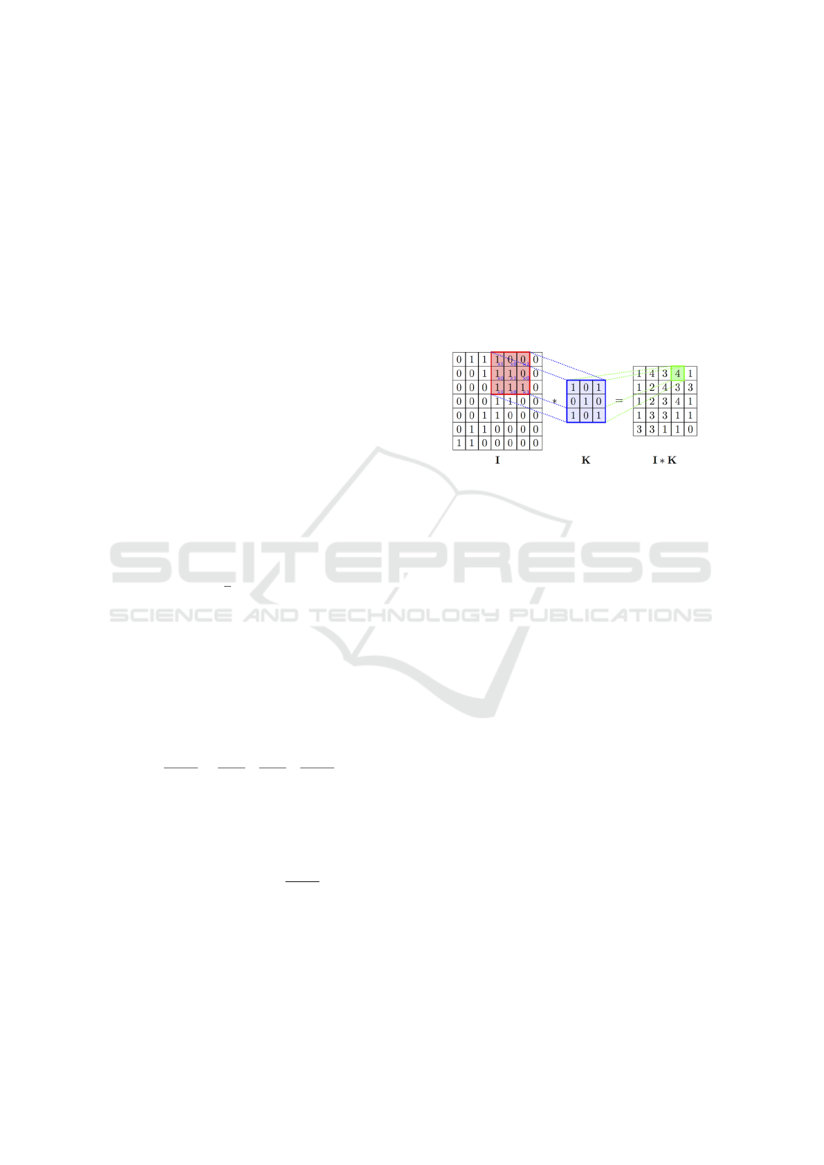
Convolution layers are used to analyze parts of or
reduce the dimensionality of the input by applying a
linear filter to the input matrix. This is done by ite-
rating a kernel matrix (K) of the dimension k
1
∗ k
2
through the whole input matrix (K). The kernel ma-
trix represents the weights and is updated through
backward propagation. Figure 1 shows an example
of convolution operation based on the formula:
(I ∗ K)
i j
=
k
1
−1
∑
m=0
k
2
−1
∑
n=0
∗I(i + m, j + n)K(−m,−n)
After applying the convolution operation to the input
matrix, the bias value adds the possibility of moving
the curve of the activation function in the x-direction
and improve the prediction of the input data. Sub-
Figure 1: Example of a convolution operation (Veli
ˇ
ckovi
´
c,
2017).
sequently, the non-linear function adds some non-
linearity. Without that, the output would be a linear
combination of the input, and the network could only
be as powerful as the linear regression. Doing that al-
lows the network to learn functions with higher com-
plexity than linear ones (Nair and Hinton, 2010).
Pooling layers reduce the complexity and compu-
tation demands of the network, without involving any
learning. The layer uses the given input matrix and
creates a more compact representation of the matrix
by summarizing it. It typically works with a 2 ∗ 2
window matrix iterating over the input matrix without
overlapping. There are different kinds of pooling lay-
ers such as max-pooling or average-pooling. Using
max-pooling, the highest value of the four cells ser-
ves as the representation of those cells instead of an
average value.
Dropout layers randomly ignore a percentage of
the input neurons. This process only happens during
the network training, for validation and prediction. As
(Srivastava et al., 2014) showed, applying the dropout
mechanism in a network increases the training du-
ration but also increases the generality and prevents
overfitting the network to the training set. The dro-
pout procedure changes for each training sequence,
as it is dependent on the input data.
Flatten layers reduce the dimensionality of the in-
put. For example, they convert a tri-dimensional input
(12x4x3) into a bi-dimensional ones (1x144).
Dense layers are used to change the size of the gi-
ven input vector. This dimensionality change is pro-
DATA 2018 - 7th International Conference on Data Science, Technology and Applications
120

duced by connecting each row of the input vector to
an element of the output vector. This linear transfor-
mation uses a weight matrix to control the strength of
the connection between one input neuron and the out-
put neurons. Like convolutional layers, a bias value
is added after the transformation, and an activation
function adds some non-linearity. Dense layers are
often used as the last layer of the network to reduce
the dimensionality to usable dimension to get the pre-
diction value, for example, with the softmax activation
function, mostly used to get the predicted category in
a classification task.
The choice of using CNNs in this work is derived
from the traditional way this architecture is used in
NLP applications: to extract position-invariant featu-
res from each input data set, for example in image
processing. Conversely, RNNs (and their variant
LSTM) are good at modeling units in sequence, which
are usually temporally controlled (Yin et al., 2017).
As we did not model our input data being tempo-
rally dependent, but rather segmented the raw text
into chunks of predefined length, we adopted a non-
recursive approach,to benefit from the better perfor-
mances of a pure feed-forward networks, such as the
convolutional ones.
3 CONCEPTUAL MODEL
The experimental setup has the following characteris-
tics: The input of the neural network is represented by
a list of all N-grams extracted from the English Wiki-
pedia corpus, with a length of 7, encoded into a fixed
300-dimensional matrix by the word embedding mo-
del. The neural network is trained by using the set of
Wikipedia page titles as the gold standard for deciding
whether a sequence of words represents a concept: if
an N-gram corresponds to a Wikipedia entry title, the
training signal to the neural network is 1; else 0. The
output of the neural network, for each N-gram, is a
prediction of whether it represents a concept or not,
together with the probability. The goal is to maxi-
mize the precision of the concept list, to obtain a high
hit rate. The objective is to support automatic docu-
ment tagging with N-gram concept extraction. Eva-
luation of the neural network’s output success, again,
uses Wikipedia page titles. If the neural network clas-
sifies a word sequence as a concept, then this is a true
positive (TP) if there is a Wikipedia page with this
title; otherwise, it is a false positive (FP). If the net-
work classifies an N-gram as a non-concept, then this
is a true negative (TN) if there is no Wikipedia entry
with that name, or else it is a false negative (FN).
3.1 Network Architecture
Figure 2 shows the NN network architecture.
Figure 2: Basic Network Structure.
The input matrix is fixed to the dimensions 7×300
and contains the vector representation of the N-grams.
Since the network needs a fixed input size, the matrix
will be filled up with zero vectors. After specifying
the input of the network, the convolution layers start
analyzing the given data. For this purpose, two se-
parate network paths analyzing the data in the hori-
zontal and vertical directions are built. Each of those
two paths includes multiple convolution layers with
different dimensions to gather different perspective of
the data. All layers use a one-dimensional convolu-
tion layer that maps the two-dimensional inputs to a
one-dimensional output. As shown in Figure 3 ver-
tical convolution layers use filters with a fixed width
of 300 and a dynamic height (here 2,3, 4). On the
Figure 3: Vertical Convolution Layer.
other hand horizontal convolution Layers (shown in
Figure 4) are using a fixed height of 7 and a dynamic
width (with typical values 30, 50,70). The rectified
linear unit (ReLU), f (x) = max(0, x), serves as acti-
vation function for all filters, to add non-linearity to
the output. Since the output dimension of the convo-
lution layers is related to the filter size, the outputs of
the filters are not balanced. For example, a vertical
filter of size 2 × 300 produces an output vector of size
6 while an output vector for a filte size of 4 × 300 has
Concept Extraction with Convolutional Neural Networks
121
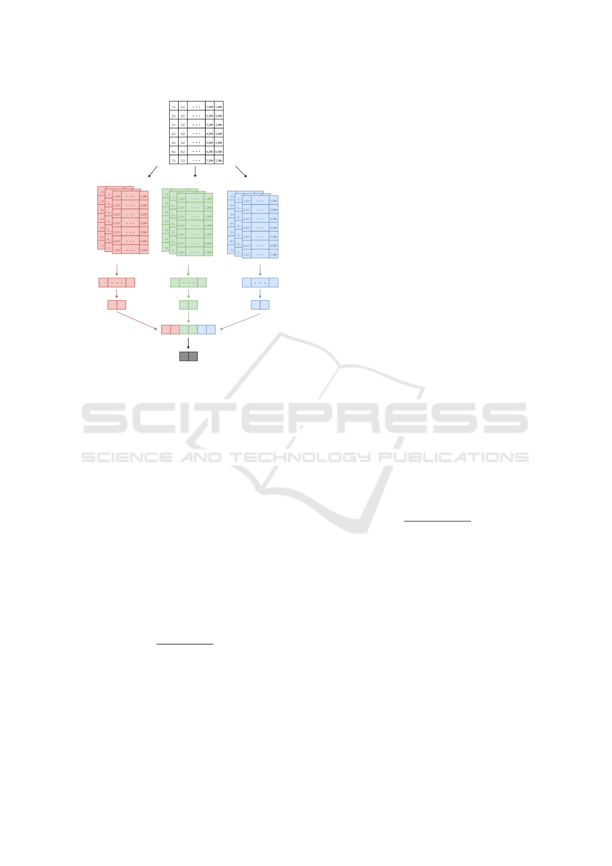
Figure 4: Horizontal Convolution Layer.
length of 4. To deal with this aspect, after the pool-
ing layers have reduced the complexity, some dense
layers decrease the length of the output vector of each
horizontal and vertical filter to 2. They also use the
ReLU function as their activation function.
After reducing the dimensions, a merge layer joins
all vectors of the horizontal and vertical paths. Then,
the dimensionality of both resulting vectors will be
reduced again to 2 by the usage of a dense layer. This
eventually results in two vectors of length 2, 1 for the
horizontal path and 1 for the vertical path.
To get the final prediction for the input, a merge
layer joins both vectors of the two paths into one vec-
tor with length 4. Subsequently, a final dense layer
uses the softmax function (as seen in Equation 4) to
reduce the dimensions to 2. It squashes all values of
the result vector between 0 and 1 in a way that the
sum of these elements equals 1. The processed result
represents the probability of one input N-gram being
marked as concept.
exp(a
k
( ¯x))
∑
j
exp(a
j
( ¯x))
(4)
3.2 Word Embedding as N-Gram
Features
For NLP applications, the choice of a word embed-
ding plays a fundamental role, while also holding
some contextual information about the surrounding
words. This information could enable an NN to re-
cognize N-grams that it has never seen in this se-
quence, thanks to a previously seen similar combina-
tion. For example, the training on the term ”Univer-
sity of Applied Science” could also enable the recog-
nition of ”University of Theoretical Science”, thanks
to the commonalities within the N-gram structure and
despite their semantic differences.
The following two models generate the vector re-
presentation of a word: Word2Vec is a pre-trained
300-dimensional model without additional informa-
tion hosted by (Google, 2013). Word2Vec-plus is our
extended version of the pre-trained model from (Goo-
gle, 2013). It uses words with a minimum frequency
of 50, extracted from a data set with 5.5 million Wiki-
pedia articles. To get a vector representation v
u
for an
unknown word, the approach uses the average vector
representation of the surrounding four words, if they
have a valid vector, or the zero vector, if they are also
unknown (shown in Equation 5).
v
u
= avg(
2
∑
i=−2
i6=0
v
i
)
(
v
i
, w
i
= known word
v
i
=
0, w
i
= unknown word
(5)
After averaging the unknown vector for one occur-
rence, the overall average v
n
will be recalculated. As
shown in Equation 6, the existing average v
n−1
will
be multiplied by the previous occurrences w
n−1
of the
word and added to the vector calculated in Equation 5.
This value will be divided by the number of previous
occurrences plus 1, to get a updated overall average
for the unknown word. This variant of the average
calculation prevents large memory consumption for
an expanding collections of vectors.
v
n
=
v
n−1
∗ w
n−1
+ v
u
w
n−1
+ 1
(6)
4 EXPERIMENTAL EVALUATION
Different network configurations were tested to find
the best model for classifying concepts and non-
concepts in our test case, according to the concpe-
tual model described in the previous section. Figure 5
shows the iterative training pipeline:
1. Initially, the features of all N-grams found in the
English Wikipedia corpus were calculated by ex-
tracting the corresponding word vectors from the
embedding model.
2. Afterwards, the data set was separated into the
training set (80%) and the test set (20%).
3. The training process used the training set to ge-
nerate the extraction network. In this phase, the
DATA 2018 - 7th International Conference on Data Science, Technology and Applications
122
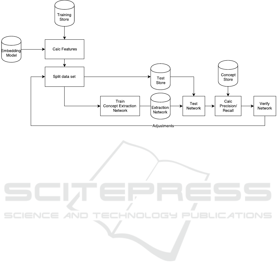
Figure 5: The adopted training pipeline.
network was trained to recognize n-grams that are
likely to represent a Wikipedia page title, based
on their structure.
4. The prediction of the resulting network was based
on the test set. During this process, all items of
the test set were classified either as concepts or
non-concepts.
5. The verification of the network was based on pre-
cision, recall, and f1 metrics calculated during the
previous evaluation.
6. Based on the performance comparison of a run
with the previous ones, either the pipeline was fi-
nished or another round was started with an upda-
ted network structure.
4.1 Data Encoding
The encoding used for presenting the data to the net-
works influences their performance, especially its abi-
lity for generalization. A good generalization depends
mainly on the following three aspects:
• Data balancing: the input data is well-balanced
by containing a similar amount of concept and
non-concept examples. The final data set con-
tains one million concepts and one million se-
lected non-concepts. These two million samples
do not fit completely into memory; thus dividing
them into 40 parts avoids a memory overflow. The
training process loads all of these parts, one by
one for each epoch.
• Data separating: existing samples are separa-
ted into the training part (80%) and the test
part (20%) to prevent overfitting of the networks.
Cross-validation gives information about the level
of generalization and mean performance. First of
all, it separates the training part into four parts
(25% of the original 80% set). Each of them is
used once as validation part, while the remaining
three parts serve as training data for the network.
The precision, recall, and f1 score give a weight
to each run of the cross-validation process of each
network. Further changes to the network structure
are based on these values to improve the perfor-
mance. Also, those metrics are used to select the
better performing and most stable networks. A fi-
nal training run on these network uses the whole
training part as input data and the quality part to
produce a final measurement of the best networks.
• Shuffling of the input data helps to get early con-
vergence and to achieve better generalization, as
also mentioned by (Bengio, 2012). For this pur-
pose, the training environment loads all training
parts in each epoch in a new random order. Furt-
hermore, it shuffles all examples inside each part
before generating the batches to send as network
inputs.
4.2 Selected Architectures
Table 1 specifies the different network configurations
adopted to investigate how vertical (v-filters) and ho-
rizontal (h-filters) filters can affect the performance of
the resulting network.
Concept Extraction with Convolutional Neural Networks
123

Table 1: Different model combinations.
Name v-filters h-filters
V3H0 (2 ,3, 4) ()
V6H0 (2 ,3, 4, 5, 6, 7) ()
V0H3 () (100, 200, 300)
V3H1 (2, 3, 4) (1)
V3H3 (2, 3, 4) (100,200,300)
V6H1 (2, 3, 4, 5, 6, 7) (1)
V6H3 (2, 3, 4, 5, 6, 7) (100, 200, 300)
V6H6 (2, 3, 4, 5, 6, 7) (10, 20, 30, 40, 50, 60)
4.3 Hyperparametrization
The intervals of the parameters shown in Table 2 are
considered during the training. The actual combina-
tion differs by use case or experiment and is based
on well-performing sets experienced during the whole
project.
Table 2: Hyperparameters.
Parameter value
Dropout 0.1-0.5
Learning Rate 0.0001, 0.0005
Epochs 100-400
Batch Size 32, 64, 128, 256
4.4 Integrated Evaluation
The evaluation was performed in two steps, based
on different degrees of integration and heterogeneous
networks configurations.
We firstly relied on the output of the already exis-
ting solution based on the part of speech (POS). This
was performed by using a restricted labeled data set,
evaluating 20,000 N-grams for each of the networks.
This is considered as a baseline comprehension mea-
surement. For this purpose, the data set contains ex-
amples that have already been labeled by the different
networks. This means the results produced by the ex-
isting solution were used as inputs. For each network
the balanced data set contains, respectively, 5,000 true
positive, true negative, false positive, and false nega-
tive examples.
Eventually, by replacing the existing approach
completely with the NN solution, we achieved a fully
integrated pipeline. For this purpose the prototype
extracts for all 130,000 N-grams — with the highest
quality — the top five keyphrases. These are chosen
out of a list of extracted concepts.
To limit the human effort in classifying the results,
we relied on the assumptions that valid concepts are
statistically present as page names (titles) into Wiki-
pedia, and that non-concepts are likely to not appear
as page titles in this source, despite the known limits
of this approach.
5 RESULTS
The evaluation of the different experiments yielded
the following observed results:
5.1 Generality
One way to measure the generality of a network
is through a k-fold evaluation. As this process is
normally computationally expensive, we reduced the
time required to do the cross-evaluation by limiting
k to the value 4 and by considering just the usage
of 100 epochs, for the training. The validity of the
last simplification is also supported by the observa-
tion that during all observed experiments, the lear-
ning curve never changed significantly after that ite-
ration, but only continued in the identified direction
towards the optimal value. The 4-fold evaluation was
run twice to gather eight runs per network. The re-
sulting values from the training phase were then used
to calculate the precision, recall, and f1 for all runs.
Figure 6 shows a summary of these training executi-
ons metrics for all networks. The majority of them
observed very close measures (limited to differences
of 0.05). This suggests that they were all stable in trai-
ning and were producing relatively general models.
However, some outliers were detected in almost all of
the models. Comparing a single set of 4-folds curves
Figure 6: 4-fold summary.
(such as on Figure 7) reveals one of those outliers.
The existence of these outliers indicates that there is
still a lack of generality within the network.
DATA 2018 - 7th International Conference on Data Science, Technology and Applications
124
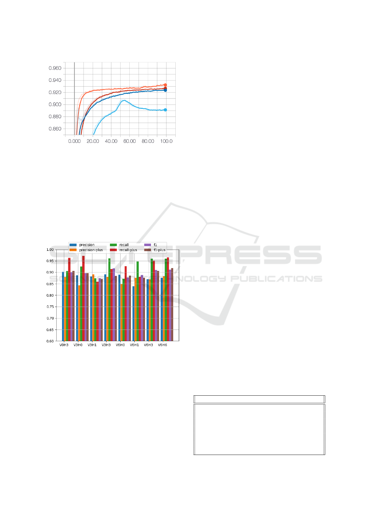
Figure 7: 4-fold precision for V6H3.
5.2 Word Embedding Comprehension
After evaluating the generality, both embedding mo-
dels Word2Vec and the extended version Word2Vec-
plus were compared. For this purpose, Figure 8
shows the different performance metrics of both mo-
dels for all network architectures. It seems that there
were no significant differences between these two
models. Nevertheless, Word2Vec-plus in combina-
tion with the V6H6 architecture gained the best per-
formance among the tested combinations. Additio-
Figure 8: Models comprehension.
nally, as shown in Figure 9, the mean learning cur-
ves of the networks based on Word2Vec-plus were
much smoother than those of the base version. One
of the purposes of the Word2Vec algorithm is to iden-
tify words that appear in a similar context (and thus
have some similarity). Looking at the additionally
generated vectors in Word2Vec-plus, it appears that is
only partly true. In fact, for words with a high fre-
quency in the text, these surroundings can degenerate
into random entries. For example, the pronoun a has
just random similar words, but the word ”Husuni”
has a high similarity with ”Kubwa” and ”Palace”.
This correct similarity indication is justified by the
facts that a palace in Tanzania exists named Husuni
Kubwa, and that the word itself is not frequent.
5.3 Vertical and Horizontal Filters
During the experiment different vertical and horizon-
tal filters were used in different models, giving the
following indications:
• By considering precision and f1, it looks like the
performance increased with the number of filters
(vertical and horizontal). On the other hand, re-
call revealed fewer peculiarities between the dif-
ferent networks but a greater variance and also the
appearance of some outliers.
• The horizontal filters show that the performance
of the model in which H = 0 is almost as good
as H = 6, but with a greater dispersion. Thus, a
larger number of vertical filters may support the
generality of the network.
5.4 Overall Performance
Figure 10 shows the resulting precision, recall, and
f1 values for all vertical and horizontal filter combi-
nations, after the 400 training epochs. Here, some
differences emerge:
• Based on precision, the V3H1 network had slig-
htly better performance than V6H6 and V3H3,
with a score of 0.8875.
• Considering the recall, on the other hand, the
V0H3 (0.9625) architecture outperformed V6H3
and V6H6.
• Using the f1 score, V0H3, V6H3, and V6H6 net-
works outperformed all others. However, among
them, none has a significantly better performance,
with all in the range from 0.91 to 0.9175.
As the N-gram length can play a role in the per-
formances, their total count and distribution between
valid and non-valid concepts in the test data set are
reported in Table 3. The unbalanced distribution is
clearly evident. In fact the performances of all net-
Table 3: Test data set distribution.
length total count concepts non concepts
1-gram 90413 91.9% 8.1%
2-gram 164463 61.2% 38.8%
3-gram 107170 21.4% 75.9%
4-gram 52997 14.3% 85.7%
5-gram 20638 11.7% 88.3%
6-gram 8217 10.9% 89.1%
7-gram 3843 8.2% 91.8%
Concept Extraction with Convolutional Neural Networks
125

Figure 9: Embedding models comprehension: Comparison of Word2Vec and Word2Vec-plus.
Figure 10: Overall performance of the tested vertical and
horizontal filters combinations in the training phase.
Figure 11: Learning curves.
works decrease as the N-gram length increases. Other
than evaluating the whole test data set at once, the
performance gaps of the different networks increased
until some networks fell below 0.5. As before, V6H6,
V6H3, and V0H3 outperformed their competitors; ad-
ditionally, V3H0 performed almost equivalently. This
suggests that they are more robust against unbalanced
data and can achieve a more stable training process.
By looking at the precision and the loss curve
(shown in Figure 11), it seems that some of the net-
works still have the potential to improve, especially
since the loss curve did not converge completely after
400 epochs. V6H3 and V3H3 might achieve better
performance as the number of epochs increases. In
contrast to those two, V6H6 seemed to reach its op-
timum at the end. V6H6 ran, in contrast to the ot-
hers, with a learning rate of 0.005 instead of 0.001.
The higher structural complexity and the correspon-
dingly higher computational complexity supports the
increased learning rate. Table 4 lists some classifica-
tion examples, separated by their membership in the
confusion matrix. True positive (TP) and true nega-
tive (TN) contain meaningful examples. The phrase
”carry out” is an example of a concept that does not
make sense out of context, but there is a Wikipedia
page about it. Similar phrases can be found from
among the FP examples, such as ”University of The-
oretical Science” and ”Mexican State Senate”: they
look like proper concepts but there is no Wikipedia
entry with that title. They were probably selected be-
cause of the similar structure to some concepts. This
also happened in the opposite direction; for exam-
ple the phrase ”in conversation with” is classified as
non-concept based on the similarity with actual non-
concepts; yet there is a TV series on BBC with the
same name.
5.5 Integration and Validation
An evaluation of each network against our initial
POS- and TF-IDF-based approach should give a fee-
ling on how well they behave, on top of the statis-
tical evaluation. The CNN approach was integrated
into the TF-IDF keyword extraction, using it as a con-
cept candidate filter in comparision to POS-based fil-
tering. For this purpose, separate data sets were used
DATA 2018 - 7th International Conference on Data Science, Technology and Applications
126
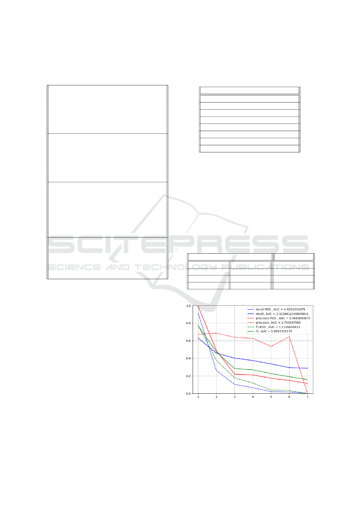
Table 4: Examples of neural network output, classified as
true positives (TP), false positives (FP), true negatives (TN),
and false negatives (FN) with regards to existing Wikipedia
page titles.
TP American Educational Research Journal
Tianjin Medical University
carry out
Bono and The Edge
Sons of the San Joaquin
Glastonbury Lake Village
Earl of Darnley
TN to the start of World War II
must complete their
just a small part
a citizen of Afghanistan who
itself include
NFL and the
a Sky
FP Regiment Hussars
University of Theoretical Science
Inland Aircraft Fuel Depot
NHL and
Mexican State Senate
University of
Ireland Station
In process
FN therefore it is
use by
in conversation with
Council of the Isles of Scilly
Xiahou Dun
The Tenant of Wildfell Hall
to compute the labels given by the NN and then used
as sources for the POS/TF-IDF performance compa-
rison. Eight data sets (one for each NN configuration)
were initialized with a precision and recall of 0.5. Ta-
ble 5 shows the general performance of CNN base
concept extraction on these validation data sets. As
can be seen, the precision and recall values were sig-
nificantly lower than those obtained from the training
phase.
Figure 12 lists the resulting precision and recall of
evaluating only the top five keywords for different N-
gram lengths. In general, all of the networks perfor-
med slightly better regarding the f1 score. Conside-
ring recall, they all outperformed the POS approach,
but they obtained lower values regarding precision.
Looking at the N-Gram length level reveals additio-
nal differences (Figure 12) when comparing the mean
performance of the initial approach (POS) to those of
various networks. Especially in consideration of the
recall value, the POS-based concept extraction almost
missed all concepts with greater length. On the con-
trary, the different networks could catch them but at
the price of lower precision. Overall the different net-
works had better f1 values than the POS approach.
Table 5: CNN models’ results to the validation set.
Network precision recall f1
V6H6 0.650 0.323 0.432
V6H3 0.659 0.326 0.436
V3H0 0.731 0.317 0.442
V0H3 0.694 0.331 0.448
V6H0 0.702 0.334 0.452
V3H3 0.649 0.348 0.453
V6H1 0.668 0.353 0.462
V3H1 0.640 0.366 0.466
Table 6 shows the total precision metrics for di-
ferent NN configurations, compared to the best, the
worst and the average configuration of POS-based
concept filtering. Over all, the POS approach can re-
ach a higher maximal precision.
Table 6: Performance metrics for a combination of CNN-
based N-gram concept recognition with a TF-IDF-based re-
levance ranking, based on extracting the top 5 keyphrases,
applied to a corpus of 100K Wikipedia articles, compared
to the minimal, maximal and average precision of different
configurations of POS-based concept recognition. The pre-
cision or hit rate represents the average percentage of top
5 key-phrases per document that correspond to a Wikipedia
concept.
CNNs POS
V3H1 0.942 V6H0 0.931 max 0.984
V6H6 0.941 V6H3 0.937 min 0.823
V3H3 0.940 V0H3 0.932
V6H1 0.938 V3H0 0.927 mean 0.927
Figure 12: Performances, ith respect to N-gram length, of
the CNN and POS approaches integrated with TF-IDF ran-
king and top-five cutoff.
Concept Extraction with Convolutional Neural Networks
127

6 DISCUSSION
The above experiments present a way to recognize
word sequences as candidate concepts for key-phrase
extraction.
For the application of concept extraction to au-
tomatic tagging of documents, we are interested in
high precision because false positives decrease user
acceptance of the system. Regarding the recall and
f1, CNN solutions performed well on the classifica-
tion task, but none of the tested configurations was
able to achieve a precision scores as high as the re-
call. This behavior is a disadvantage, especially for
preventing false positives, which is important for user
acceptance of automatic tagging.
In the training phase, the outcome demonstrated
a precision of between 80 and 90 perent. However,
integrating the CNN concept extraction into the initial
prototype and thus applying it to a different validation
dataset only showed a precision of between 60% and
80%, on average. So there was an overfitting taking
place when training the CNN.
Anyhow, combined with a TF-IDF based rele-
vance ranking, the top five n-gram concepts calcula-
ted for wikipedia articles showed a greater precision
of up to 94%. This means that on average, out of four
documents, each with five automatically extracted top
keywords, only one document contained an N-gram
that is not a Wikipedia entry title.
Yet, the precision of the best performing POS con-
cept filtering together with TF-IDF relevance ranking
and top five cutoff was even better with 98%. Howe-
ver, this precision decreased drastically with increa-
sing number of words in the N-grams. The POS ap-
proach filtered out many N-grams with greater N. The
CNN-based approach recognized much more N-gram
concepts, which can be seen in the recall curves in
Table 6 by comparing the blue straight line represen-
ting CNN-recall) with the blue dotted line represen-
ting POS-recall.
Using Wikipedia as gold standard, there is a ge-
neral acknowledgment that each page certainly repre-
sents a concept. Of course, the opposite is not true: if
there is no Wikipedia entry for a phrase, it could still
be valid concept. Although we did not run analyses
in this respect, (Parameswaran et al., 2010) provided
contributions through crowd-sourced effort, demon-
strating that the percentage of valid concepts not ex-
isting as Wikipedia pages is less than 3% of all the
n-grams in the FN category.
As seen, the networks had weaknesses regarding
generality. They were able to perform on unseen data
as well as they did on the validation set during the
training. However, when repeating the training for
the same network, they revealed outliers. Too much
dropout overall or in the wrong position could have
been one of the sources for this behavior. Thereby,
the networks may have received too much random-
ness and were unable to learn the small essential diffe-
rences between the word vectors. Furthermore, some
dropout could have been replaced by the usage of L1
and L2 regularization. This would polarize the con-
nections by manipulating the weights (Ng, 2004) to-
wards a simpler network with either heavy weights or
no weights between neurons.
There are several aspects to be considered for furt-
her research projects: a) Experimenting with different
word features could increase the performance signifi-
cantly. b) Instead of using a balanced list of concepts
and non-concepts, the training data could be genera-
ted by going through the text copus word by word.
Thus, the network would be trained with n-grams in
the sequence they appear in the text. Thus, frequent
N-grams would be getting more weight. c) Changing
the input consideratiosn and using a recurrent neural
network instead of a CNN could improve the results.
Compared to the latter, RNNs do not require a fixed
input and was found to somehow outperforms it in
some NLP tasks. d) One network could be trained
per N-gram length, so that the network does not need
to take all the different distributions into account at
once.
REFERENCES
Bengio, Y. (2012). Practical recommendations for gradient-
based training of deep architectures. CoRR, abs/
1206.5533.
Dalvi, N., Kumar, R., Pang, B., Ramakrishnan, R., Tom-
kins, A., Bohannon, P., Keerthi, S., and Merugu, S.
(2009). A web of concepts. In Proceedings of the
Twenty-eighth ACM SIGMOD-SIGACT-SIGART Sym-
posium on Principles of Database Systems, PODS
’09, pages 1–12, New York, NY, USA. ACM.
Das, B., Pal, S., Mondal, S. K., Dalui, D., and Shome, S. K.
(2013). Automatic keyword extraction from any text
document using n-gram rigid collocation. Int. J. Soft
Comput. Eng.(IJSCE), 3(2):238–242.
F
¨
urnkranz, J. (1998). A study using n-gram features for text
categorization. Austrian Research Institute for Artifi-
cal Intelligence, 3(1998):1–10.
Google (2013). Googlenews-vectors-negative300.bin.gz.
https://drive.google.com/file/d/0B7XkCwpI5KDYNl
NUTTlSS21pQmM/edit. (Accessed on 01/15/2018).
Hughes, M., Li, I., Kotoulas, S., and Suzumura, T. (2017).
Medical text classification using convolutional neural
networks. arXiv preprint arXiv:1704.06841.
Joulin, A., Grave, E., Bojanowski, P., and Mikolov, T.
(2016). Bag of tricks for efficient text classification.
arXiv preprint arXiv:1607.01759.
DATA 2018 - 7th International Conference on Data Science, Technology and Applications
128

Kalchbrenner, N., Grefenstette, E., and Blunsom, P. (2014).
A convolutional neural network for modelling senten-
ces. CoRR, abs/1404.2188.
Kim, Y. (2014). Convolutional neural networks for sentence
classification. arXiv preprint arXiv:1408.5882.
Liu, Y., Shi, M., and Li, C. (2016). Domain ontology
concept extraction method based on text. In Compu-
ter and Information Science (ICIS), 2016 IEEE/ACIS
15th International Conference on, pages 1–5. IEEE.
Lopez, M. M. and Kalita, J. (2017). Deep learning applied
to NLP. CoRR, abs/1703.03091.
Mikolov, T., Chen, K., Corrado, G., and Dean, J. (2013).
Efficient estimation of word representations in vector
space. arXiv preprint arXiv:1301.3781.
Nair, V. and Hinton, G. E. (2010). Rectified linear units im-
prove restricted boltzmann machines. In Proceedings
of the 27th international conference on machine lear-
ning (ICML-10), pages 807–814.
Ng, A. Y. (2004). Feature selection, l 1 vs. l 2 regulari-
zation, and rotational invariance. In Proceedings of
the twenty-first international conference on Machine
learning, page 78. ACM.
Parameswaran, A., Garcia-Molina, H., and Rajaraman, A.
(2010). Towards the web of concepts: Extracting con-
cepts from large datasets. Proceedings of the VLDB
Endowment, 3(1-2):566–577.
Rong, X. (2014). word2vec parameter learning explained.
arXiv preprint arXiv:1411.2738.
Siegfried, P. and Waldis, A. (2017). Automatische gene-
rierung plattform
¨
ubergreifender wissensnetzwerken
mit metadaten und volltextindexierung. http://www.
enterpriselab.ch/webabstracts/projekte/diplomarbeiten/
2017/Siegfried.Waldis.2017.bda.html.
Srivastava, N., Hinton, G., Krizhevsky, A., Sutskever, I.,
and Salakhutdinov, R. (2014). Dropout: A simple way
to prevent neural networks from overfitting. The Jour-
nal of Machine Learning Research, 15(1):1929–1958.
Veli
ˇ
ckovi
´
c, P. (2017). Deep learning for complete
beginners: convolutional neural networks with ke-
ras. https://cambridgespark.com/content/tutorials/
convolutional-neural-networks-with-keras/index.html.
(Accessed on 01/29/2018).
Westphal, C. and Pei, G. (2009). Scalable routing via
greedy embedding. In INFOCOM 2009, IEEE, pages
2826–2830. IEEE.
Yin, W., Kann, K., Yu, M., and Sch
¨
utze, H. (2017). Compa-
rative study of cnn and rnn for natural language pro-
cessing. arXiv preprint arXiv:1702.01923.
Zhang, Q., Wang, Y., Gong, Y., and Huang, X. (2016).
Keyphrase extraction using deep recurrent neural net-
works on twitter. In EMNLP.
Concept Extraction with Convolutional Neural Networks
129
