Steps Towards a Balance between Adequacy and Time Optimization in

Agent-based Simulations

A Practical Application of the Temporality Model Time Scheduling Approach

Tahina Ralitera, Nathan Aky, Denis Payet and R

emy Courdier

Laboratoire d’Informatique et de Math

ematiques, University of Reunion Island, France

Keywords:

Simulation Platform, Scheduler, Time Management, Temporality, Comparison, SimSKUAD.

Abstract:

Simulation models are often used as decision support tools. They intend to imitate real world complex phe-

nomena or processes. For this purpose, simulation platforms has the simulated models evolve by advancing a

virtual time. Thus, users could beneﬁt from shorter, but relevant simulations. The simulated time is managed

by the scheduler and how this is done could signiﬁcantly impact on the performance of the simulation plat-

form. However, conventional time scheduling approaches are still limited in some situations. The temporality

model approach was proposed as an interesting solution. It addresses a number of criteria that the classical

time scheduling approaches do not fulﬁl. In this paper, we ﬁrst describe the fundamental of the temporality

model approach. Then, we implement it in a simulation model called the SKUADCityModel. Finally, we

show the performance advantages of this type of approach.

1 INTRODUCTION

Agent-Based simulation models are usually used as

decision support tools. They allow, for example, to

evaluate the possible consequences of real projects

before their implementation in the real world. For that

purpose, a simulation platform has a simulation mo-

del evolve following a virtual time. In general, this

virtual time progresses much faster than real time.

The simulation platform part that is responsible for

this virtual time management is called the schedu-

ler. This scheduler uses different approaches among

which the most commonly used are the time-stepped,

the event-driven and the mixed approaches.

We are interested in applications on personal com-

puters and in that case, conventional time scheduling

approaches may be inappropriate or may have limits

depending on the situation. These limits could affect

the performance of the simulation platform. To ad-

dress that, (Payet et al., 2006) proposed the “tempora-

lity model” approach. This approach intends to fulﬁl

a set of criteria that the classical approaches of sche-

duler do not meet. This paper clariﬁes the fundamen-

tals of this temporality model approach, presented in

an abstract way in (Payet et al., 2006) and proposes a

practical application of it.

A set of requirements that we think an agent-based

simulation scheduler should meet are listed in the next

section. Then, we talk about the most commonly used

time scheduling approaches and their limits. Next, we

describe the temporality model approach and the per-

formance advantages of this type of scheduler appro-

ach. Finally, we end with a practical implementation.

2 RELATED WORK

2.1 Requirements

(Payet et al., 2006) list a set of requirements that a

scheduler should meet to be reasonably ﬁt for multi-

agent simulations:

1. Take into Account the Speciﬁcities of the Simu-

lated Model (Helleboogh et al., 2004):

Models can take various and complex forms. It

would be unrealistic to believe that a time ma-

nagement approach could work properly without

any consideration of these simulated model featu-

res.

2. Take into Account the Experimental Con-

straints:

A simulation often implies a shorter execution

time than real time. Thus, depending on the com-

plexity of the simulated model, the user can be

160

Ralitera, T., Aky, N., Payet, D. and Courdier, R.

Steps Towards a Balance between Adequacy and Time Optimization in Agent-based Simulations - A Practical Application of the Temporality Model Time Scheduling Approach.

DOI: 10.5220/0006904601600166

In Proceedings of 8th International Conference on Simulation and Modeling Methodologies, Technologies and Applications (SIMULTECH 2018), pages 160-166

ISBN: 978-989-758-323-0

forced to reduce the simulation execution time by

constraining the simulation platform. The more

these constraints are stronger the less precise the

results are. However, it is better than not getting

any results at all.

3. Establish a Homogeneous Management of

Time:

Sometimes the user needs a ﬂexible time sche-

duling approach that could adapt to time-stepped

and to pure event-driven simulation contexts. In

that way, all the results are obtained on the same

experimental basis and can be compared (Axtell,

2000).

4. Handle a Cumulative Characterization of

Time:

Multidisciplinary complex phenomena simulation

models could be developed by several modelers.

Most of the time, none of these modelers have the

full control over the model. Thus, it will be inte-

resting to have a cumulative time scheduling that

can be partially deﬁned by each modeler, while

remaining coherent.

5. Handle an Incremental Complexity:

Currently, we manage to obtain complex structu-

ral and behavioural description models. However

the time management is still basic. Consequently,

the simulation results seem to be limited at a le-

vel that time dimension does not allow to cross

(Amblard and Dumoulin, 2004). Thus, it could be

interesting to have a time scheduling mechanism

that could handle an incremental complexity.

6. Minimize the Impact on the Execution Perfor-

mance:

In our case, a good scheduling mechanism should

work properly with the available computing po-

wer on personal computers.

In the following subsections, we describe the three

most used types of scheduler approaches and how

they fail to address some of these requirements.

2.2 The Time-stepped Approach

Because of its ease of implementation, the time-

stepped approach is the most used approach in the

agent-based simulations. In this approach, the sche-

duler advances the simulation time by incrementing

its value by a ﬁxed duration ∆t called time-step (Fu-

jimoto, 1998). The simulated time can be represen-

ted by an axis that is discretized by ﬁxed intervals (ﬁ-

gure 1). With each time-step, all the simulation activi-

ties (agent cycle and possibly objects simulation) are

completed before advancing to the next step.

Figure 1: Time axis for time-stepped approaches.

This approach is usually easy to set up. Also, it is

convenient for one speciﬁc model composed of agents

that have homogeneous behaviour and the same acti-

vation frequency. However, it becomes unsatisfactory

in the case of highly heterogeneous agents’ behaviour.

Indeed, using an inappropriate time step value can

lead to lethargic or overactive agents. On one hand,

if the agent is activated too infrequently, his actions

seem slowed. On the other hand, if the agent is activa-

ted too often, his actions seem accelerated. The both

cases may lead to erroneous simulation results.

To address that, a solution consists in setting a

time step value that is equal to the smallest time inter-

val required. Then, to avoid hyperactivity, the agents

that require a bigger time step value have to explicitly

become inactive during the intermediate time steps

that are not relevant for them. The opposite appro-

ach is not possible. Indeed, an agent can slow down

his activity, but he does not have the possibility of

acting at a smaller granularity than that imposed by

the scheduler. Consequently, when only a very small

number of agents need a small time step value, the

majority of the agents spend most of their time to be-

come inactive. (Michel, 2004) concludes that using a

regular discretization of time is unsatisfactory when

the simulated model needs to take highly heterogene-

ous agent actions (from the frequency point of view)

into account.

To summarize, this approach does not take the

speciﬁcity of any simulated model into account.

2.3 The Event-driven Approach

In this approach, the simulation axis is continuous but

the state of the system changes discretely at precise

time called events (Anagnostou et al., ). An event can

be deﬁned as the description of the agents’ behavi-

our activation conditions at a particular time. Its rele-

ase date can be calculated depending on the nature of

these conditions. Thus, the simulation consists in exe-

cuting an orderly list of events. The time axis can be

represented by a chained event list that are not equit-

ably spaced (ﬁgure 2).

This approach is suitable in case of highly hete-

rogeneous agents. However, the user of the platform

does not have any control over the simulated time. He

is not able to force the simulator to reduce the simu-

lation execution time. However, for large-scale simu-

Steps Towards a Balance between Adequacy and Time Optimization in Agent-based Simulations - A Practical Application of the

Temporality Model Time Scheduling Approach

161

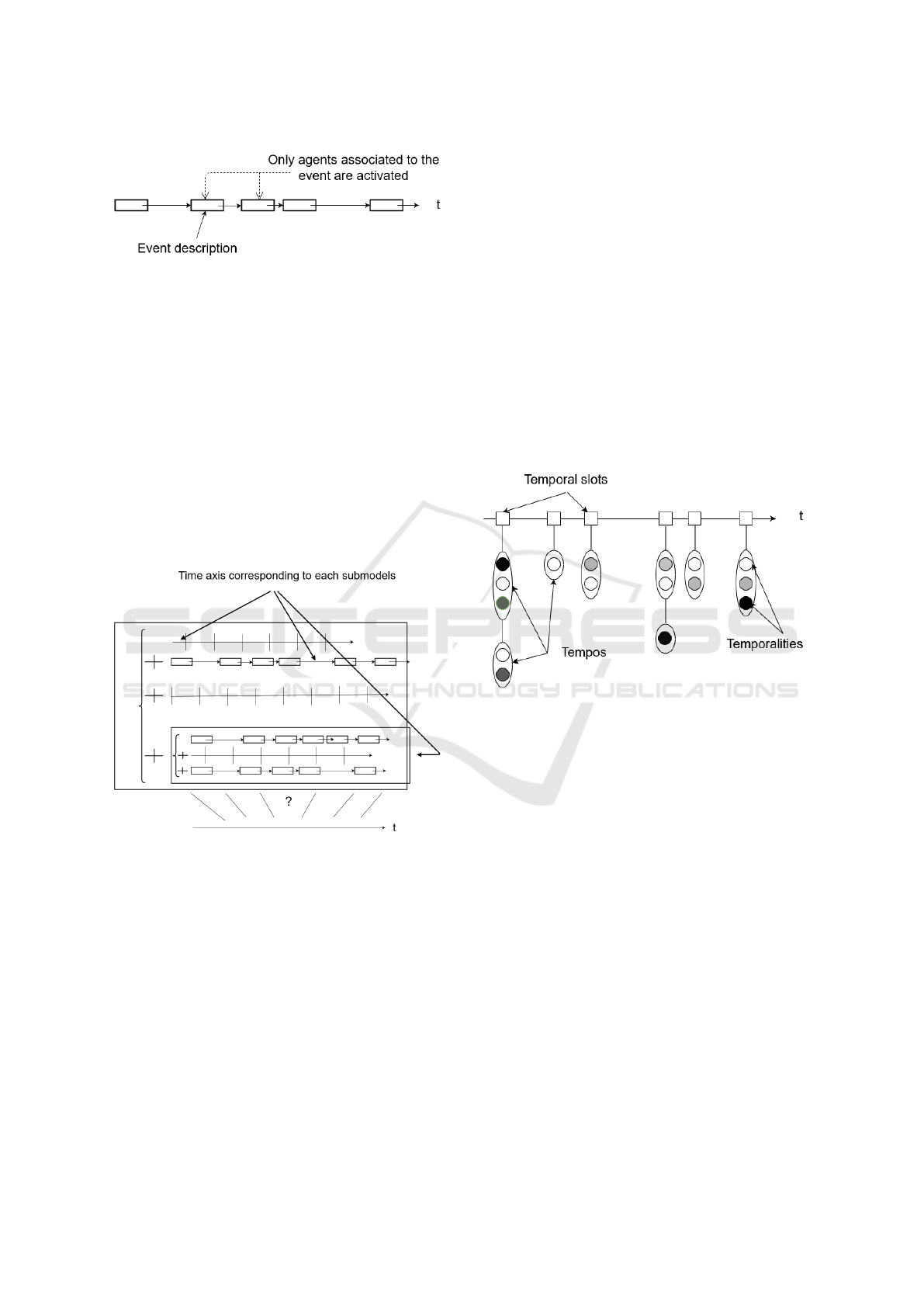
Figure 2: Time axis for event-driven approaches.

lations, this possibility of making compromises is es-

sential.

Moreover, the simulated time can take very com-

plex forms. Thus, the calculations made by the simu-

lator can be rather substantial. Consequently, it could

require lots of computational power.

2.4 The Mixed Approach

The mixed approaches propose to split the simulated

model into sub-models. To each sub-model is asso-

ciated the most appropriate type of scheduler. The

resulting time management system is the combina-

tion of the different chosen schedulers. Consequently,

there is no global time axis (ﬁgure 3).

Figure 3: Time axis for mixed approaches.

This lack of global vision is a limit if we want to

make analysis of the simulation time. Moreover, any

attempt to inﬂuence the simulated time structure in

order to reduce the execution time duration is prohi-

bited.

2.5 The Temporality Model Approach

In multi-agent systems, an agent typically has some

autonomy over the characterization of its state and its

behaviour. In the same way, in the temporality mo-

del approach, the agent describes its own activation ti-

mes itself. This kind of scheduler is focused on needs

which are directly expressed by the agents.

The agents needs are expressed using a data struc-

ture called “the temporality”.

A temporality t speciﬁes a point on the time axis

where an agent wants to be activated. t can be deﬁned

by the tuple (Payet et al., 2006):

t = {id, d, f , p, v} (1)

where:

• id is the identiﬁer of the temporality.

• [d, f ] is the time interval during which the tempo-

rality can be activated.

• [p] is the time period, i.e. the time interval bet-

ween two executions of this temporality (p = 0 if

the action is only executed once).

• v is the variability. It deﬁnes the accuracy below

which the temporal occurence remains valid.

Figure 4: Time axis for the temporality model approach.

The agents behaviour activation time is equal to x =

d + p ∗ k, where k is an integer such as 0 ≤ k ≤ n and

n is the biggest integer that veriﬁes (d + p ∗ n) = f

(Payet et al., 2006).

The agents deﬁne their temporalities during the si-

mulation initialization. Afterward, they will be able to

redeﬁne or create new temporalities any time. In that

case, the scheduler immediately processes the creati-

ons and modiﬁcations, then updates the time axis.

One particularity of the temporality model ap-

proach is the ability to allow the user to inﬂuence

the simulated time structure by adding time con-

straints. These time constraints are the minimum

time-step, the default time period and the variability.

• The minimum time-step ∆t

min

, indicates that two

distinct activation dates should be separated by a

duration at least equal to the value of ∆t

min

. If

such a situation occurs during the analysis of the

temporalities, the scheduler will use the variabi-

lity parameter v of each of the temporalities to

determine if they should be separated from each

other or grouped together on the same date.

SIMULTECH 2018 - 8th International Conference on Simulation and Modeling Methodologies, Technologies and Applications

162

• The default time period value that is used by

agents that do not deﬁne any temporalities during

the initialization of the simulation.

The scheduler processes the temporalities using

two data structures (see ﬁgure 4):

• The temporal slot: a precise time when the sche-

duler must activate the agent’s behaviour.

• The tempo: a set of temporalities which are loca-

ted on the same time slot and which have the same

time period. This time period characterizes the

tempo. It means that all the temporalities it con-

tains have the same activation rhythm. The sche-

duler advances the simulated time from a time slot

to another. At each time slot, all the tempos are

processed. That produces the execution of all the

behaviours associated with the temporalities they

contain.

(Payet et al., 2006) propose the temporality model

as a solution that fulﬁl the criteria cited in section 2.1:

1. By deﬁnition, the temporality model approach is

based on the speciﬁcity of the simulated model.

2. The temporality model approach allows the user

to inﬂuence the simulated time structure by ad-

ding time constraints. This is done by varying the

minimum time step, the default period and the va-

riability.

3. This approach allows for ﬁne management of

complex agents in term of diversity of activation

rhythm, but does not complicate the simple agents

management. The simple agents do not have to

deﬁne any temporality and the system will auto-

matically assign them a default one (deﬁned at the

beginning by the user). Thus, in the extreme ca-

ses, on one hand, if no agent deﬁnes a temporality,

we automatically fall back into a time-stepped ap-

proach. On the other hand, if all the agents are

complex and express a large number of tempo-

ralities, we end up with an event-driven type of

scheduling.

4. For complex agents, the writing of the behavior

can be done by different developers (Each speci-

alist in his ﬁeld). How then determine the glo-

bal temporal operating mode of the agent? Who

has the competence? The granularity of the tem-

porality model approach is the activities. Conse-

quently, each developer participates in the deﬁni-

tion of the temporality of the agent as for the deﬁ-

nition of its behavior.

5. In this approach, the agents temporal needs are

expressed at the level of the agents’ activities. It

is possible to relate a speciﬁc temporality with

each distinct activity. Also, the complexity of

these temporalities can be accentuated at the same

time that the behavior to which they are attached

is made even more complex. Thus, this appro-

ach supports an incremental complexiﬁcation in

the same way as that which can be achieved at the

level of writing the agents’ behavior.

6. A way to implement a temporal model is the use

of time slots and tempos. These can take the form

of a linked list that manages the simulated time

and that determine the agents’ activation time. As

we have experienced, and as has been shown by

(Lawson and Park, 2000), such a data structure

can be optimized with the algorithms of (Henrik-

sen, 1983) so the resulting execution time remains

around that of the time stepped approach.

(Payet et al., 2006) use assumptions and illustra-

tive examples to demonstrate the advantages of the

use of the temporality model approach. They made a

comparative study between the different classical ap-

proaches and the temporality model. In this article,

we support their demonstration with a practical appli-

cation.

3 CASE STUDY

The proposed case study is about agent-based simula-

tion of individual transport. This is done for the city

of Saint-Denis, capital of Reunion Island, a French

island in the Indian Ocean.

In this simulation model, agents are vehicle ow-

ners. The model uses activity-based approach so

agents move from a place to another following their

activity schedule. Thus, travels result from personal

activities (work, shopping, leisure, going home) that

individuals need or wish to perform.

3.1 The Agent Model

In our simulation model, an agent is a vehicle owner.

His goal is to achieve all his activities using the vehi-

cle at his disposal. The activity proﬁle AP

for each

group i of vehicle owners is deﬁned with a list of 3-

tuples:

= (ACT

, MDT

, PD

) (2)

Where ACT

represents the activity j, MDT

the mean

departure time, and PD

the probability of departure

for the activity j.

Steps Towards a Balance between Adequacy and Time Optimization in Agent-based Simulations - A Practical Application of the

Temporality Model Time Scheduling Approach

163

3.2 The Environment Modeling

Elements

The environment in which the agents are situated and

act is represented by a collection of entities. These

entities represent fragments of the real environment.

Its deﬁnition is done using Geographic Information

System (GIS) composed of the following layers:

• The building layer that is a set of polygon entities

and that represents administrative boundaries.

• The road layer that is composed of polyline en-

tities and that represents the road network along

which the agents move.

• The areas of interests layers, represented by poly-

gon or point entities. They represent the location

of the home, the workplace, the leisure, the com-

mercial or the industrial places.

The simulation model takes shape ﬁles and statistical

data as input. They are used at the different level of

the simulation model such as for environment model-

ling or for the calculation of the population distribu-

tion.

In the following sections we will show how we

built this simulation model upon the SimSKUAD si-

mulation platform.

4 THE SKUADCityModel

4.1 SKUAD

SKUAD stands for “Software Kit for Ubiquitous

Agent Development”. This free multi-platform tool-

kit is still being developed. It allows us to create

multi-agent systems using Java language. It has been

developed since 2013 by the Collective Adaptive Sys-

tems Research Group in the Laboratory of Mathema-

tics and Computer Science (LIM) at the University of

Reunion Island. The idea comes from the observation

of the outburst of the Internet of Things, and the ne-

cessity to have a software that can make this mass of

objects more consistent. For that purpose, SKUAD

can operate in an ambient (agents can operate in our

real environment) and in a simulated mode.

4.2 The SimSKUAD Simulation

Platform

The SimSKUAD is the simulated operating mode of

SKUAD. In this mode, the agents evolve following a

simulated time. Devices constituting the agent’s en-

vironment are virtual. The SimSKUAD uses the tem-

porality model as a default time scheduling approach.

However, its architecture is ﬂexible enough to allow

us to easily replace the scheduler. Thus, we were also

able to implement the time-stepped approach.

Different optional modules have already been de-

veloped for SimSKUAD. Examples are Mod2D allo-

wing agents simulations in a continuous space envi-

ronment or ModGrid which allowing agents simulati-

ons in a discrete space environment. More details can

be found on the SKUAD website (Payet, 2018).

In this paper, we focus in a module called Mod-

GIS that allows agents to evolve in Geographical In-

formation System (GIS) kind of environment. For

that, ModGIS uses the GeoTools library (Turton,

2008).

The SKUADCityModel is built upon the ModGIS

module of the SimSKUAD simulation platform. In

our experiments, we implemented two different types

of scheduler: a time-stepped approach and a tempora-

lity model approach. In the next section, we compare

the experimental results obtained from these two ty-

pes of approaches.

5 COMPARISON OF THE

DIFFERENT APPROACHES

In this section, we illustrate the advantages of the tem-

porality model approach against classical approaches

by experiments on the SKUADCityModel. For that

purpose, we make two types of manipulations:

• The ﬁrst manipulation is to vary the experimen-

tal constraints (time step duration and the vari-

ability) from 0% to 100%. In this way, we show

how the simulation duration can be reduced de-

pending on the used time scheduling approach.

• The second one is a scaling up test. For that pur-

pose, we vary the number of agents from 1000 to

10,000 moving moving over simulated 12 hours.

In this way, we show how the simulation model

can scale up depending on the used time schedu-

ler approach.

Remark: We chose to not make implementation

of the event-driven or the mixed approaches because

they are not appropriate if we want the users to have

control over the simulated time (see section 2.1).

For this experiment, we run the two simulation

models on a personal computer with the following

conﬁguration : ﬁfth generation Intel core i5, 16 gi-

gabytes of RAM, Solid State Drive.

SIMULTECH 2018 - 8th International Conference on Simulation and Modeling Methodologies, Technologies and Applications

164

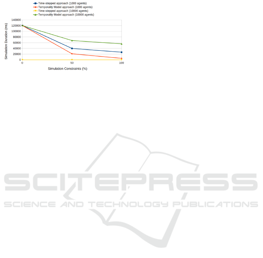
Figure 5: Execution duration performance of each schedu-

ling mode for 1000 then 10000 agents.

Figure 5 shows the results of the ﬁrst experiments

we carried.

First, in the case where no experimental constraint

is applied (0%) and for 1000 agents, we can see

that the simulation execution durations are almost the

same for the two approaches. However, when we vary

the experimental constraints (50%, 100%), we can see

a sharp decrease of the simulation execution duration.

This decrease is greater in case of the use of the tem-

porality model approach.

Second, we note a difﬁculty of scaling up in case

of the time-stepped approach. Indeed, the results

show that when using the time-stepped approach, the

maximum number of agents supported by the SKU-

ADCityModel does not exceed 10,000. In the ﬁgure

5, the yellow curve on 0ms indicates a crash due to

an out of memory error. This is a problem we do not

encounter, at least up to 10,000 agents, when we use

the temporality model approach.

Finally, the performances remain acceptable and

the simulation execution times are less than ﬁve mi-

nutes. These results are in line with the demonstra-

tions made in (Payet et al., 2006). That shows the

performance advantages of this type of scheduler ap-

proach. Especially, it allows the user to have control

over the simulated time. Moreover, it allows to scale

while maintaining acceptable performance.

6 CONCLUSION AND FURTHER

WORK

Agents scheduling management is a critical process in

simulation platforms. Unfortunately, all the conventi-

onal approaches have limits in some situations. From

case to case, these limits could be very restrictive.

(Payet et al., 2006) proposes the temporality model

approach as a possible solution that addresses some

of these limits. They demonstrate that by illustrative

examples based on theoretical assumptions.

In this paper, we show that the temporality model

meets requirements that we think agent-based simu-

lation of urban and transport system should fulﬁl:

• It takes into account the speciﬁcities of the si-

mulated model and can automatically adapt to

them. Indeed, in the case of homogeneous agents,

the temporality model works like a time-stepped

approach. In the case of highly heterogeneous

agents, it works like an event-driven approach.

• It takes into account the experimental con-

straints as it allows to vary a set of parameters in

order to shorten the simulation execution duration

for example.

• It ensures a homogeneous management and

acumulative characterization of time because

all the agents’ actions are based on the same vir-

tual timeline.

• It activates agents who need to be awake only

when they need to be. Consequently, it handles

an incremental complexity and minimizes the

impact on the execution performance.

We support these assumptions with practical appli-

cations. For that, we implemented the time-stepped

approach and the temporality approach in a same si-

mulation model called the SKUADCityModel. Then,

we compared the two implementations based on the

execution time performance and the ability of the si-

mulation model to scale.

The results are in agreement with the theoretical

demonstrations that have already been made in (Payet

et al., 2006). In our experiments, we used the Sim-

SKUAD simulation platform, that is still under deve-

lopment and that has an architecture that seems to be

different compared to classic agent-based simulation

platform. As further work, it could be interesting to

see if the architecture of the SimSKUAD simulation

platform also affects the performance of the simula-

tion.

The demonstration done in this paper is limited to

a comparison with the classical time management ap-

proaches. However, the relevance of the temporality

model approach should be further assessed with more

advanced mechanisms such as the time-stepped load

balancing approach described in (Wu et al., 2015) In

addition, it would be interesting to increase the perfor-

mance already obtained using the GPU calculation, as

proposed in the paper (Song et al., 2017).

ACKNOWLEDGEMENTS

The research in this paper was supported by the

egion R

eunion, the L’Or

eal-UNESCO for women in

Steps Towards a Balance between Adequacy and Time Optimization in Agent-based Simulations - A Practical Application of the

Temporality Model Time Scheduling Approach

165

science fellowship and the town of Saint-Denis. The

authors thank the reviewers for their comments.

REFERENCES

Amblard, F. and Dumoulin, N. (2004). Mieux prendre

en compte le temps dans les simulations individus-

centr

ees. 11

emes Journ

ees de Rochebrune, pages 13–

26.

Anagnostou, A., Meskarian, R., Robertson, D., and Fak-

himi, M. Introduction to discrete-event simulation:

how it works. In Welcome to the 2018 Operational Re-

search Society Simulation Workshop (SW18), page 13.

Axtell, R. L. (2000). Effects of interaction topology and

activation regime in several multi-agent systems. In

Multi-Agent-Based Simulation, Second International

Workshop, MABS 2000, Boston, MA, USA, July, 2000,

Revised and Additional Papers, pages 33–48.

Fujimoto, R. M. (1998). Time management in the high level

architecture. Simulation, 71(6):388–400.

Helleboogh, A., Holvoet, T., Weyns, D., and Berbers,

Y. (2004). Extending time management support for

multi-agent systems. In Multi-Agent and Multi-Agent-

Based Simulation, Joint Workshop MABS 2004, New

York, NY, USA, July 19, 2004, Revised Selected Pa-

pers, pages 37–48.

Henriksen, J. O. (1983). Event list management - a tutorial.

In Proceedings of the 15th conference on Winter si-

mulation, WSC 1983, Arlington, VA, USA, December

12-14, 1983, pages 543–551.

Lawson, B. G. and Park, S. (2000). Asynchronous time

evolution in an artiﬁcial society model. J. Artiﬁcial

Societies and Social Simulation, 3(1).

Michel, F. (2004). Formalisme, outils et

ements

ethodologiques pour la mod

elisation et la simula-

tion multi-agents. (Formalism, tools and methodologi-

cal elements for the modeling and simulation of multi-

agents systems). PhD thesis, Montpellier 2 University,

France.

Payet, D. (2018). Ofﬁcial website of skuad. http://skuad.

onover.top/, Last accessed on 2018-15-07.

Payet, D., Courdier, R., Ralambondrainy, T., and S

ebastien,

N. (2006). Le mod

ele

a temporalit

e: pour un

equilibre

entre ad

equation et optimisation du temps dans les si-

mulations agent. In Systemes Multi-Agents, Articula-

tion entre l’individuel et le collectif - JFSMA 2006 -

Quatorzieme journees francophones sur les systemes

multi-agents, Annecy, France, October 18-20, 2006,

pages 63–76.

Song, X., Xie, Z., Xu, Y., Tan, G., Tang, W., Bi, J., and Li,

X. (2017). Supporting real-world network-oriented

mesoscopic trafﬁc simulation on GPU. Simulation

Modelling Practice and Theory, 74:46–63.

Turton, I. (2008). Open Source Approaches in Spatial Data

Handling. Springer, Berlin, Heidelberg.

Wu, Y., Song, X., and Gong, G. (2015). Real-time load ba-

lancing scheduling algorithm for periodic simulation

models. Simulation Modelling Practice and Theory,

52:123–134.

SIMULTECH 2018 - 8th International Conference on Simulation and Modeling Methodologies, Technologies and Applications

166