
Integrated Guidance, Navigation, and Control System for a UAV in a
GPS Denied Environment
Ju-Hyeon Hong
1
, Chang-Kyung Ryoo
2
, Hyo-Sang Shin
1
and Antonios Tsourdos
1
1
School of Aerospace, Transportation, and Manufacturing, Cranfield University, College Road, MK43 0AL, Cranfield, U.K.
2
Aerospace Engineering, Inha University, 100 Inharo, Namgu, 22212, Incheon, Republic of Korea
Keywords: GPS Denied Environment, Indoor Flight, Integrated Guidance Navigation and Control System, Visual
Guidance and Control.
Abstract: This paper proposes an integrated guidance, navigation, and control system for operations of a UAV in GPS
denied environments. The proposed system uses a sensor combination, which consists of an image sensor
and a range sensor. The main idea of the system developed is that it replaces the conventional navigation
information with the measurement from the image processing. For example, it is possible to substitute the
look angle and look angle rate from the image sensor for the conventional navigation information like the
relative target position and the body angular rate. As the preliminary study, the integrated guidance and
control system is designed with a nonlinear back-stepping approach to investigate the possibility of the
proposed system. And the proposed integrated guidance and control system is verified by the numerical
simulation.
1 INTRODUCTION
The large scale of small Unmanned Aerial Vehicle
(UAV) applications has proliferated vastly within
the last few years. The operational experience of
UAVs has proven that their technology can bring a
dramatic impact to military and civilian areas. There
are numerous potential applications under
consideration and being studied at the moment.
One of interesting aspects in applications of
small UAVs is that they might need to be operated
in a GPS denied environment such as inside a
building. In such a case, the most common
navigation system in aerospace, namely INS/GPS
system is not applicable and hence other means of
navigation should be sought for.
Simultaneous localization and mapping (SLAM)
and the visual odometry are two common alternative
navigation systems that could be implemented in a
GPS denied environment or indoor environment.
(Achtelik et al., 2009; Ahrens et al., 2009; Alarcon
et al., 2015; Blösch et al., 2010; Çelik and Somani,
2009; Chowdhary et al., 2013; Ghadiok et al., 2011;
Kendoul et al., 2009) Although they can provide
reasonable performance, they might be subject to a
relatively complex sensor combination or require
high computational power. Since the operations of
small UAVs are constrained by limited payload and
power, applying the two systems might become
restricted in practice.
Under these backgrounds, this paper aims to
develop a new navigation system that is suitable for
operations of a small UAV in a GPS denied
environment. The focus of the development is to test
how far we can push in terms of the types and
number of sensors required. The guidance,
navigation and control (GNC) systems are the main
driver determining sensor requirements. Therefore,
this study also focuses to come up with an
appropriate GNC system for the sensor combination
selected.
The sensor combination proposed and tested in
this paper consists of only an image sensor and a
range sensor. We intend to investigate whether it is
possible to abandon the need for an inertial
measurement unit (IMU), which plays the most
crucial role in navigation, up to the best of our
knowledge. Note that the proposed sensor
combination cannot provide all information required
for the conventional GNC systems. Therefore, this
paper also develops an integrated guidance and
control (IGC) system that requires the navigation
information obtainable from the proposed sensor
440
Hong, J-H., Ryoo, C-K., Shin, H-S. and Tsourdos, A.
Integrated Guidance, Navigation, and Control System for a UAV in a GPS Denied Environment.
DOI: 10.5220/0006908204400447
In Proceedings of the 15th International Conference on Informatics in Control, Automation and Robotics (ICINCO 2018) - Volume 2, pages 440-447
ISBN: 978-989-758-321-6
Copyright © 2018 by SCITEPRESS – Science and Technology Publications, Lda. All rights reserved
combination. The feasibility of the proposed
approach is investigated through initial theoretical
analysis and numerical simulations.
The rest of this paper is organised as follows. In
section 2, the mathematical models for UAV
dynamics and relative navigation information are
presented. Section 3 introduces the structure of the
integrated guidance, navigation, and control system,
which is a key contribution of this paper. To verify
the proposed integrated guidance and control
system, the results of the numerical simulation are
presented in section 4. Conclusion of this paper is
given in section 5.
2 PROBLEM DEFINITION
2.1 6-DOF Dynamics of the UAV
To design the guidance and control system, 6-DOF
dynamics are formulated. The mathematical models
are based on following assumptions.
The body and propeller of a quadcopter are
rigid and symmetric.
The thrust force is proportional to the square
of motor’s speed.
The earth rotation can be ignored.
The inertial coordinate system is a flat earth
model.
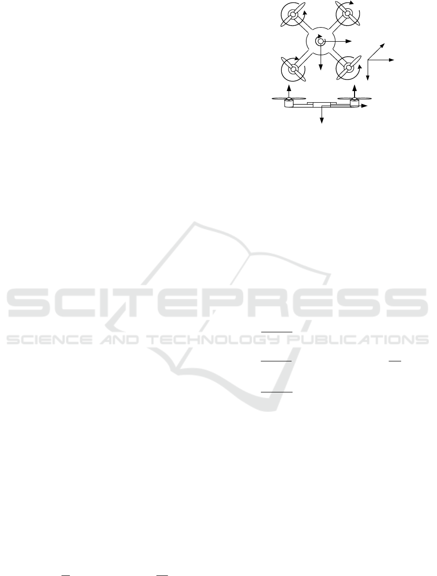
The coordinate system and forces for the UAV
model are shown in Figure 1. The inertial frame is a
north-east-down frame (n-frame). And the body
frame (b-frame) is a fixed frame of the body of the
UAV.
Let
T
nnn
xyz
rrr
and
[]
T
φ
θ
ψ
denote a
position vector in n-frame and an attitude angle
vector respectively. The aerodynamic friction
coefficients are and
tr
K
K respectively. The mass
and vector of the moment of inertia are
and , ,
x
xyyzz
mIII
respectively. The thrust force
and vector of the moment are respectively
and
T
xyz
TMMM
. The vector of body
angular rate is
[]
T
pqr
. The dynamic model of
the UAV is given as follows:
0cc
0ssccs
csc ss
nn
xx
nn
t
yy
nn
zz
rr
K
T
rr
mm
rg r
θψ
φθψ φψ
φθψ φψ
=− − +
+
(1)
b
x
b
y
×
b
x
b
z
n
x
n
y
n
z
1
Ω
4
Ω
3
Ω
2
Ω
14
,
F
F
23
,
F
F
Figure 1: The coordinate system for a quadcopter.
1ts tc
0c s
0ssc csc
r
pp
qRq
rr
φθφθφ
θφφ
ψφθφθ
=−+
(2)
where
22
/c/
0
t
0
//
0
/ /
r
sc c
cts
Rs c
ts c tc c
cc sc
φθθ φθθ
θ
φφ
θ
φφ
φφ φφ
θ φ θθ θ φ θθ
φ
θ
φφ
θ
φ
+−
=− −
+−
(3)
0/
0/
/
yy zz
xx
xxx
zz xx
r
yyy
yy
zzz
xx yy
zz
II
qr
I
pMIp
II
K
qprMIq
Im
rgMIr
II
qr
I
−
−
=++−
−
(4)
The forces of motors are given by :
2
, ( 1, 2, 3, , 4)
ii
F k i and=Ω =
(5)
where
and
i
k Ω are the motor parameter and the
rotational speed of the i-th motor. The thrust force
and moment can be expressed by the forces of the
motors:
1
2
3
4
11 1 1
x
y
z
TF
M
F
ll l l
M
F
llll
M
F
cc c c
−−
=
−−
(6)
where
and lc
are the distance of the moment
arm and the drag factor.
Integrated Guidance, Navigation, and Control System for a UAV in a GPS Denied Environment
441
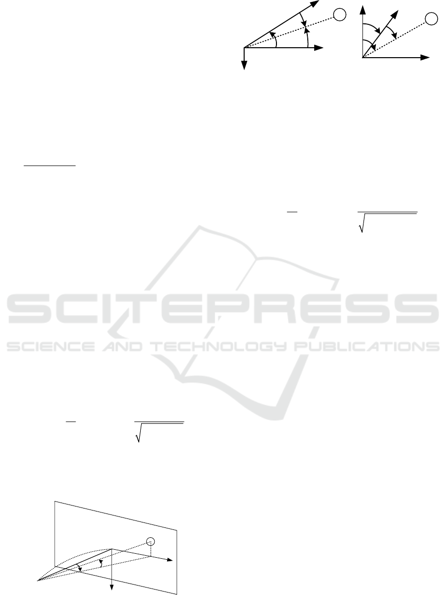
2.2 Relative Navigation Information
from Camera Frame
This section introduces the process for relative
navigation information in the camera frame (c-
frame). The relative navigation information can be
expressed by a target vector from UAV to the target
in the c-frame. Figure 2 shows the target vector in c-
frame. The focal length of the camera and the look
angle vector are
and , f
θψ
λλ
respectively. The
unit target vector in c-frame is given as:
cos cos
tan
tan sec
c
fcc
ufsc
f
fs
ψθ
ψθ
ψψθ
θψ θ
λλ
λλ
λλλ
λλ λ
==
−−
(7)
The unit target vector in the b-frame can be
expressed as the unit vector in the look angle frame (
λ
-frame).
cs0c0s 1
sc0010 0
001s0c 0
cc
c s
s
TT
b
u
ψψ θ θ
ψψ
θθ
θψ
θψ
θ
λλ λ λ
λλ
λλ
λλ
λλ
λ
−
=−
=
−
(8)
The unit target vector in c-frame and the unit
target vector in b-frame are the same. Therefore the
look angle can be obtained by the target vector in c-
frame.
()
11
2
2
tan , tan
c
c
y
z
c
y
r
r
f
fr
ψθ
λλ
−−
−
==
+
(9)
The main idea of the proposed the GNC system
is based on the physical characteristic of the look
angle.
ψ
λ
θ
λ
f
c
y
c
z
Target
Figure 2: The target information in camera frame.
θ
σ
ψ
σ
n
x
n
z
b
x
θ
λ
θ
b
x
n
y
n
x
ψ
λ
ψ
Target
Target
Figure 3: Definition of the LOS angle and look angle.
Let us define the LOS angle to investigate the
characteristic of the look angle. The relationship
between the LOS angle, the look angle, and the
attitude angle is shown in
Figure
3. Let define LOS angles
,
θψ
σσ
to
describe the target vector in the n-frame.
() ()
11
22
tan , tan
n
n
y
z
n
nn
x
xy
r
r
r
rr
ψθ
σσ
−−
==
+
(10)
From the LOS angle, the target vector in the n-
frame can be calculated directly. However, by using
the fixed image sensor, the UAV can obtain the
target vector in the b-frame. It means that the look
angle describes not only the variation of the target
relative position, but also the variation of the attitude
angle. If the pitch and yaw plane can be decoupled
by stabilizing roll axis, the look angle can be defined
as follows:
θθ
ψψ
λσθ
λσ
ψ
=−
=−
(11)
When the UAV moves slowly, the attitude angles
of the UAV are small. It means that the look angles
are nearly the same as the LOS angles. Therefore the
look angle can replace the LOS angle at slow speed.
Moreover the look angle rate can be described by the
derivative of eq.(11):
θθ
ψψ
λσθ
λσ
ψ
=−
=−
(12)
As shown in eq.(12), the look angle rates include
the LOS rate and the attitude angle rate. For this
reason, if the look angle rates are stabilised to zero,
the body angular rates are also conversed to zero. By
theses physical characteristics of the look angle, the
look angles and the look angle rates can be replaced
with the LOS angle and the body angular rate
respectively. In the next section, the GNC system,
which is based on these characteristic, is introduced.
ICINCO 2018 - 15th International Conference on Informatics in Control, Automation and Robotics
442
3 INTEGRATED GUIDANCE,
NAVIGATION AND CONTROL
(IGNC) SYSTEM
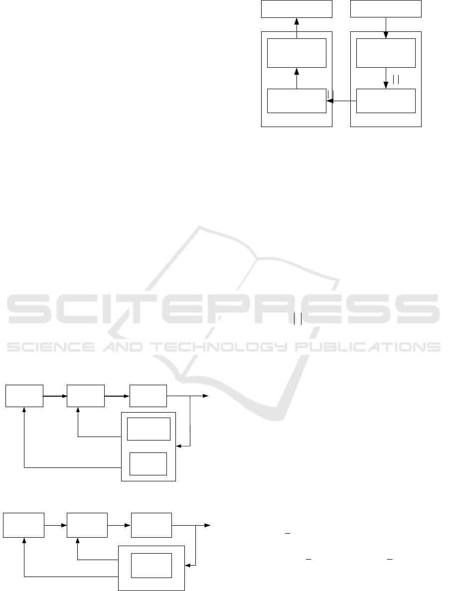
The general system framework of the conventional
guidance and control is shown in Figure 4.
Normally, the guidance and navigation system
utilizes four types of sensors, i.e., a gyroscope, an
accelerometer, a magnetometer, and a GPS. On the
other hand, this paper proposes to use an image
sensor and a range meter for our proposed guidance
and navigation system to allow operation of such
system in a GPS-denied environment. The structure
of the proposed guidance and control system is
shown in Figure 5. The proposed guidance and
control system utilizes the relative information
measured by the image sensor and the range meter.
The navigation filter, then provides the information
required for the new guidance and navigation.
The detailed structure of the IGNC system is
given in Figure 6. The target vector in c-frame and
the relative distance are measured by the image
sensor and the range sensor in the target tracking
system. In addition, the target images are used for
estimating the attitude angles by the image
processing algorithm. The outputs of the target
tracking system are used for the measurement of the
relative navigation filter. Moreover the outputs of
the relative navigation filter are used in the proposed
integrated guidance and control (IGC) system.
Finally the IGC system calculates the thrusts of the
UAV.
AutopilotGuidance
UAV
Dynamics
Gyroscope
Accelerometer
magnetometer
GPS
,, ,
b
ω
φ
θ
ψ
,
nn
vr
GPS/INS
Figure 4: The conventional guidance and control system.
AutopilotGuidance
UAV
Dynamics
Image sensor&
Range sensor
,,,
λ
φ
θ
ψ
Relative Navigation filter
,
nn
vr
Figure 5: The proposed guidance navigation and control
system.
Integrated
guidance and
controller
Image processing
Integrated GNC
Image sensor &
range sensor
Target tracking system
Target
Relative
navigation filter
,
nn
rv
ˆˆ
ˆ
, , p
θ
ψ
λλ
UAV
1234
, , ,
F
FFF
ˆˆ
ˆ
,,
φ
θ
ψ
ˆˆ
ˆ
,,
φ
θ
ψ
, , r
θ
ψ
λλ
,
c
rr
Figure 6: Integrated control and guidance system.
Since the scope of this paper is to confirm the
possibility of the IGC system, the relative navigation
filter is regarded as the ideal model in the numerical
simulation. In following sub-sections, the structures
of the relative navigation filter and the IGC system
are presented.
3.1 Relative Navigation Filter
The relative navigation filter estimates the relative
velocity, the look angle rate and the roll rate. The
relative position can be expressed as:
cc cs s
T
nn
b
rCr
θψ θψ θ
λλ λλ λ
=−
(13)
where
n
b
C
is a coordinate transformation matrix
from the b-frame to the n-frame. Since the relative
velocity, the roll rate and the look angle rate are the
derivatives of the relative position, the roll angle,
and the look angle, these parameters can be
estimated by the simple alpha-beta filter. Therefore
the state vector of the relative navigation filter is
given as
T
nnnnnn
xxyyzz
X
rvrvrv p
λλ φ
=
and the measurement vector of the relative
navigation filter is given as
T
nnn
xyz
Z rrr
λ
φ
=
. The propagation model
and update model of the relative navigation filter can
be expressed as:
() ( ) ( )
ˆ
ˆ
11Xk Xk FXk=−+ −
(14)
() () () ()
()
ˆ
X
kXkKZkHXk=+ −
(15)
where
K
is the filter gain matrix. The system
matrix
F
and the measurement matrix
H
are given
as :
Integrated Guidance, Navigation, and Control System for a UAV in a GPS Denied Environment
443

1 00000000
0100000000
001 000000
0001000000
00001 0000
0000010000
0000001 00
0000000100
000000001
0000000001
dt
dt
dt
F
dt
dt
=
(16)
1000000000
0010000000
0000100000
0000001000
0000000010
H
=
(17)
where
dt
is the time step.
3.2 Integrated Guidance and Control
(IGC) System
As the dynamics of the UAV are nonlinear, a
nonlinear back-steeping approach is applied for IGC.
Note that the back-stepping approach designed in
this paper is based on the method developed in
(Madani and Benallegue, 2006). The control input
vector is the derivatives of the thrusts of the four
motors and it is given as
1234
T
uFFFF
=
.
The dynamic equations are expressed in the state-
space form as follows:
()()()
()()()
()()()
1
2
02356 057 03
3
4
1 3467 1 3 1 7
5
6
2 3467 2 3 2 7
71234
, , , ,
, , ,
, , ,
T
nn
xy
T
nn
xy
T
T
T
n
z
T
n
z
T
xvv
xvv
f xxxx g xx x
x
x
fxxxx gx x
xv
xv
fxxxx gx x
xFFFF
ρ
φθ
φθ
ρ
ψ
ψ
ρ
=
=
=+
=
=
=+
=
=
=+
=
(18)
where
()
0
1234
0
0
03
0
3
0
n
x
t
n
y
v
K
f
v
m
s
c
FFFF
g
cs
m
s
cs
xc
J
ss cc
x
ψψ
ψψ
φ
ρ
φθ
ρφ
φθ φθ
=−
+++
=−
−
=
∂
==
−
∂
(19)
()
()
()
()
()
()
1
1234
1
1
1234
1
1234
17
1
7
1
ˆ
ˆ
0
0
1
0
0
xx yy
zz yy
r
xx zz
yy
zz
xx
yy
st
p
II
qr I I
fK
c
pr I I
I
cF F F F
tc
s
I
I
st
g
I
c
lF F F F
lF F F F
x
ll
J
x
θ
φθ
φ
λ
θφ
φ
φθ
φ
ρ
ρ
−
−
=−
−
−+−
+
−
=
+−−
=
−−+
∂
==
∂
ll
llll
−−
−−
(20)
()
()
()
2
123 4
1
2
1234
2
1234
0
0
/
ˆ
0
ˆ
ˆ
0
0
00
/
0
/0 0
00
t
n
z
yy xx
zz
r
yy
zz
K
f
v
g
m
cc
pI I
I
K
lF F F Fsc
I
cc I
g
cc m
cF F F F
FFFF
J
θ
ψ
φθ
λ
λ
φθ
φθ
φθ
ρ
−
=− +
−
+−
−−+
+
=
−
−+−
=
+++
()
27
2
7
1111
x
cccc
x
ρ
∂
−−
==
∂
(21)
The final control law can be expressed as :
ICINCO 2018 - 15th International Conference on Informatics in Control, Automation and Robotics
444
()
()()
()( )
()()
()
()()
111 1 1
1
20 11 21210
1
30012 320 2
1
41020 434 31
55555
1
62 5 5 65652
34
122
1
1
22 2
2
0
0
dd
d
T
T
dd
d
T
vAx x x
vg x x Avx vf
vJgvx Av v
vgJv Avx vf
vAxxx
vg x x Avx vf
vx
g
Jv
g
u
J
ρ
ρ
−
−
−
−
×
−
×
=−+
=−+−+−
=−+−+
=−+−+−
=−+
=−+−+−
−
=
4
56 6
41
7
62
v
xv
v
A
v
ρ
ρ
+
−
−
+
−
(22)
where
[]
()
[]
()
[]
()
[]
()
[]
()
[]
()
[]
()
1112 22
333444
555666
77777
,
,
,
A diag a a A diag a a
A diag a a A diag a a
A diag a a A diag a a
Adiagaaaa
==
==
==
=
(23)
The stability of the control structure is analysed
by Lyapunov stability theory in (Madani and
Benallegue, 2006). If the roll angle and pitch angle
are between
/2
π
±
, the whole system is
asymptotically stable. In the look angle rate
feedback loop, the rate limiter is applied, and the
range of rate limiter is ±0.5.
In the next section, the numerical simulation
results are presented to verify the IGC.
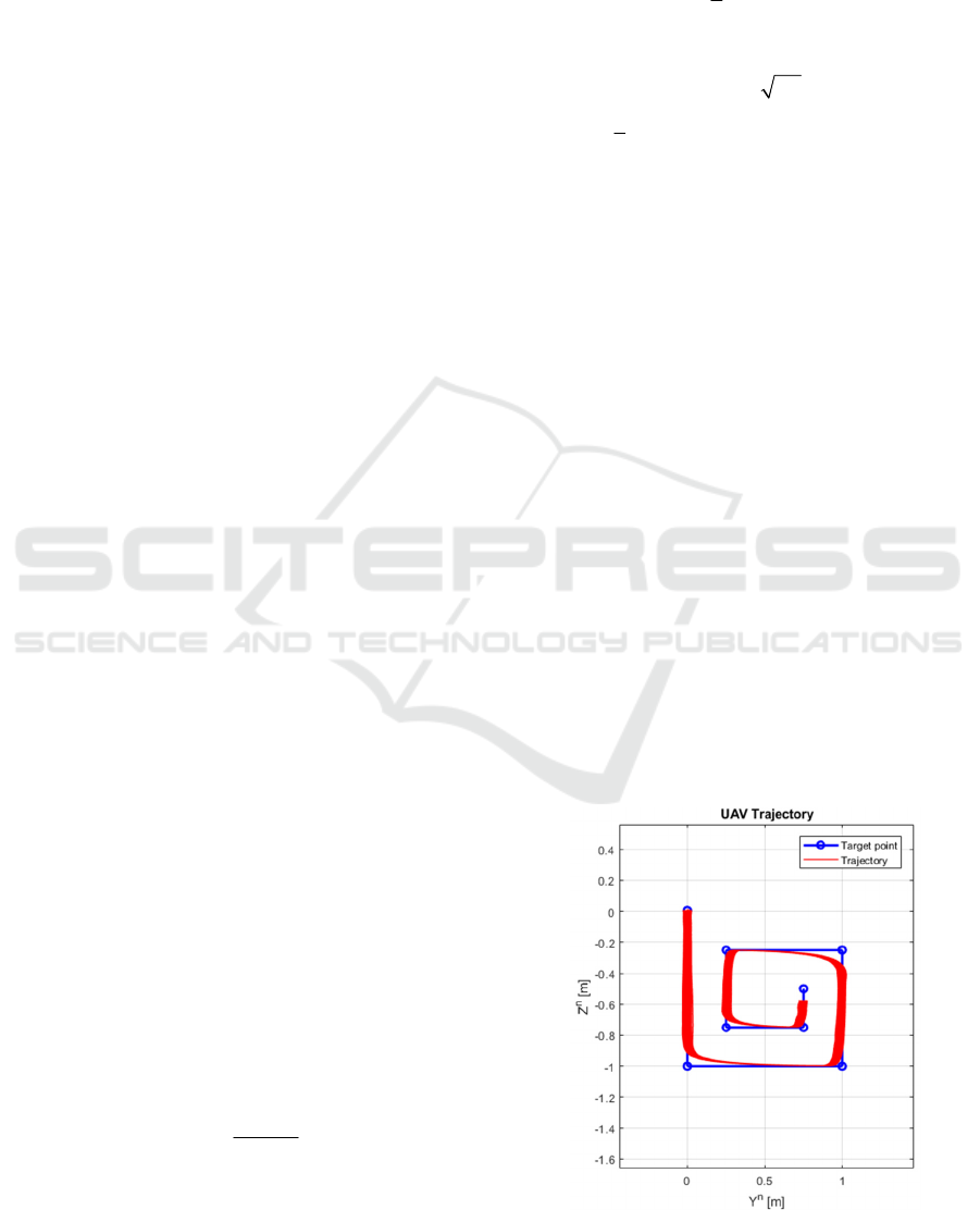
4 NUMERICAL SIMULATION
For the numerical simulation, a scenario is designed
for the indoor precise inspection. A UAV moves
toward the inspection panel and keeps the 30 cm
distance in the x axis, and tracks the target points in
the y and z axes. It is assumed that the eight target
points are detected as shown in Figure 7 and the
reference trajectory is generated by the target points.
The desired target point changes every 7.5 s and a
transient function is applied to generate the reference
trajectory. The transient function is given as:
()
()
4
1
1
Gs
s
=
+
(24)
To investigate the nature of the IGC, the target
tracking system and the relative navigation filter are
regarded as the ideal models in the numerical
simulation. However, for the realistic simulation, the
look angle rate is assumed to contain a bias and
noise:
() () ()
()
()
()
0
0
ˆˆ
~0.4/s, 0.4/s
~0, 0.1/s
kk Qk
Urad rad
Qk N rad
λλλ
λ
=++
−
(25)
where
()
k
λ
is an ideal look angle rate of k-th
step which is calculated by the geometric equation,
0
ˆ
λ
is a bias term which is generated by the uniform
distribution and it is generated in the run-wise, and
()
Qk
is a Gaussian random noise and it is generated
in the path-wise.
Figure 7-Figure 11 show Monte-Carlo simulation
results under the errors of the look angle rates, with
150 runs. Note that the Figure 7 depicts the results of
all 150 runs of Monte-Carlo simulation and others
depict the mean and ±1σ standard deviations. Figure
7 shows the trajectories of the UAV and Figure 8
depicts the tracking errors. Since the waypoint
changes before the UAV reaches the target point, the
tracking errors are increasing in the middle.
However, the tracking errors converges to zero
gradually. The additional tracking errors, which are
caused by the look angle rate errors, are less than 5
cm and these errors are negligible. Basically, the
additional manoeuvring errors occur due to the
replacement from the body angular rates to look
angle rates. As shown in Figure 8, the additional
manoeuvring errors are observed as the biased mean
values and the maximum tracking error caused by
using the look angle rates is below 2 cm.
Figure 7: The trajectory of UAV.
Integrated Guidance, Navigation, and Control System for a UAV in a GPS Denied Environment
445
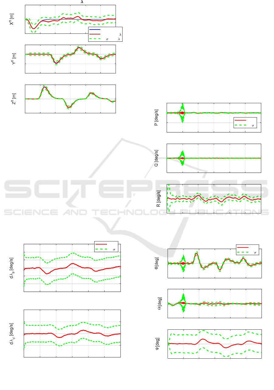
Figure 8: The history of the tracking error by
λ
errors.
The tracking errors in the x and y axes are larger
than the tracking error in the z axis because the body
dynamics of the x and y axes is an under-actuated
mechanical system. In addition, since the control
equation for the x and y axes include the Jacobian
matrix about the nonlinear equation, it affects the
stability under the noisy condition. As a result, the
stability in the x and y axes is relatively more
sensitive than the stability along the z axis.
However, the tracking errors are below 5 cm during
the total flight phase which is reasonable for the
indoor inspection.
Figure 9: The history of the look angle rates.
Figure 9-Figure 11 show the time histories of the
look angle rates, body angular rates and Euler angles
respectively. Before the UAV reaches the desired
distance in the x axis, the body attitudes are
fluctuating. After the UAV reaches the desired
distance in the x axis, attitude in each axis becomes
stable. The yaw angles have the bias error as shown
in Figure 11 because the look angle rate term in the
yaw axis directly influences the yaw angle.
However, the figure show that the total amount of
tracking errors is tolerable for the indoor inspection.
In addition, the proposed IGC keeps the stable state
during the total flight phase.
Figure 10: The history of the body angular rate.
Figure 11: The history of the Euler angles.
0 102030405060
-0.05
0
0.05
Tracking error by d Errors
with PQR
mean with d
+-1 with d
0 102030405060
-0.2
-0.1
0
0.1
0 102030405060
Time[s]
-0.1
0
0.1
0 102030405060
-30
-20
-10
0
10
20
30
Look angle rate
mean
+-1
0 102030405060
Time[s]
-40
-20
0
20
40
0 102030405060
-10
-5
0
5
Body angular rate
mean
+-1
0 102030405060
-20
0
20
0 102030405060
Time[s]
-5
0
5
0 102030405060
-0.5
0
0.5
Euler angle
mean
+-1
0 102030405060
-1
0
1
0 102030405060
Time[s]
-10
0
10
ICINCO 2018 - 15th International Conference on Informatics in Control, Automation and Robotics
446

5 CONCLUSIONS
This paper proposed an IGNC system for a UAV in
the GPS denied environment. The proposed system
uses the sensor combination, which consists of an
image sensor and a range sensor. As a feasibility
study, the performance of the proposed IGC system
validated through the numerical simulation. The
relative navigation filter and the target tracking
system are assumed as the ideal models, but a
realistic error model for the look angle rates, which
are feedback to the controller, is incorporated in the
simulation-based validation.
The proposed IGC has a difference to the
conventional attitude controller in terms of the body
angular rate loop. The IGC system replaces the body
angular rate loop to the look angle rate loop since
the look angle rate can be obtained from the image
sensor without a gyroscope. Therefore, the
gyroscope is not required and we can decrease the
number of the sensors required. As a result, the
system is subject to the additional manoeuvre, which
is caused by the difference between the body angular
rate feedback and look angle rates feedback loops,
and the look angle rate errors. However, the
influence of the additional manoeuvre is small and
negligible.
We will extend the back-stepping control
structure, incorporating the look angle estimate into
the control design, to improve the performance of
the integrated system. A practical navigation filter,
which is appropriate for the integrated system, will
be designed and integrated in the whole system.
Also, the proposed IGNC will be verified thorough
flight tests.
REFERENCES
Achtelik, M., Bachrach, A., He, R., Prentice, S., Roy, N.,
2009. Stereo vision and laser odometry for
autonomous helicopters in GPS-denied indoor
environments, in: Unmanned Systems Technology XI.
International Society for Optics and Photonics, p.
733219. https://doi.org/10.1117/12.819082.
Ahrens, S., Levine, D., Andrews, G., How, J. P., 2009.
Vision-Based Guidance and Control of a Hovering
Vehicle in Unknown, GPS-denied Environments, in:
2009 IEEE International Conference on Robotics and
Automation. IEEE, Kobe,Japan, pp. 2643–2648.
Alarcon, F., Santamaria, D., Viguria, A., 2015. UAV
helicopter relative state estimation for autonomous
landing on moving platforms in a GPS-denied
scenario, in: IFAC-PapersOnLine. Elsevier Ltd., pp.
37–42. https://doi.org/10.1016/j.ifacol.2015.08.056.
Blösch, M., Weiss, S., Scaramuzza, D., Siegwart, R.,
2010. Vision based MAV navigation in unknown and
unstructured environments, in: Robotics and
Automation (ICRA). IEEE international conference,
pp. 21–28. https://doi.org/10.1109/ROBOT.2010.
5509920.
Çelik, K., Somani, A.K., 2009. Monocular vision SLAM
for indoor aerial vehicles. J. Electr. Comput. Eng.
2013, 1566–1573. https://doi.org/10.1109/IROS.
2009.5354050.
Chowdhary, G., Johnson, E.N., Magree, D., Wu, A.,
Shein, A., 2013. GPS-denied Indoor and Outdoor
Monocular Vision Aided Navigation and Control of
Unmanned Aircraft. J. F. Robot. 30, 415–438.
https://doi.org/DOI 10.1002/rob.21454.
Ghadiok, V., Goldin, J., Ren, W., 2011. Autonomous
indoor aerial gripping using a quadrotor, in: IEEE
International Conference on Intelligent Robots and
Systems. 2011 IEEE/RSJ International Conference, pp.
4645–4651. https://doi.org/10.1109/IROS.2011.60487
86
Kendoul, F., Nonami, K., Fantoni, I., Lozano, R., 2009.
An adaptive vision-based autopilot for mini flying
machines guidance, navigation and control. Auton.
Robots 27, 165–188. https://doi.org/10.1007/s10514-
009-9135-x.
Madani, T., Benallegue, A., 2006. Backstepping Control
for a Quadrotor Helicopter, in: 2006 IEEE/RSJ
International Conference on Intelligent Robots and
Systems. IEEE, Beijing, China, pp. 3255–3260.
https://doi.org/10.1109/IROS.2006.282433.
Integrated Guidance, Navigation, and Control System for a UAV in a GPS Denied Environment
447
