Scalable Supervised Machine Learning Apparatus for Computationally

Constrained Devices

Jorge L

opez

, Andrey Laputenko

, Natalia Kushik

, Nina Yevtushenko

2,3

and Stanislav N. Torgaev

SAMOVAR, CNRS, T

ecom SudParis, Universit

e Paris-Saclay, 9 rue Charles Fourier, 91000

Evry, France

Department of Information Technologies, Tomsk State University, 36 Lenin street, 634050 Tomsk, Russia

Ivannikov Institute for System Programming of the Russian Academy of Sciences,

25 Alexander Solzhenitsyn street, 109004, Moscow, Russia

Keywords:

Supervised Machine Learning, Digital Circuits, Constrained Devices, Deep Learning.

Abstract:

Computationally constrained devices are devices with typically low resources / computational power built for

speciﬁc tasks. At the same time, recent advances in machine learning, e.g., deep learning or hierarchical or

cascade compositions of machines, that allow to accurately predict / classify some values of interest such as

quality, trust, etc., require high computational power. Often, such complicated machine learning conﬁgurations

are possible due to advances in processing units, e.g., Graphical Processing Units (GPUs). Computationally

constrained devices can also beneﬁt from such advances and an immediate question arises: how? This paper

is devoted to reply the stated question. Our approach proposes to use scalable representations of ‘trained’

models through the synthesis of logic circuits. Furthermore, we showcase how a cascade machine learning

composition can be achieved by using ‘traditional’ digital electronic devices. To validate our approach, we

present a set of preliminary experimental studies that show how different circuit apparatus clearly outperform

(in terms of processing speed and resource consumption) current machine learning software implementations.

1 INTRODUCTION

Computationally constrained devices (Bormann et al.,

2014) are devices which are typically built for dedi-

cated tasks, and therefore, even if they include general

purpose processors, computationally complex opera-

tions are unfeasible. With the fast development of the

Internet of Things (IoT), constrained devices got a lot

of attention. Therefore, it is necessary to develop new

methods to reduce the complexity of computation and

at the same time provide the ﬂexibility of modern data

science.

Particularly, providing such constrained devices

with close-to-human inference approaches that use

machine learning is of great interest as IoT devices of-

ten interact with each other relaying mission-critical

operations to their peers. For example, it is typical to

use intermediate IoT devices to route the network traf-

ﬁc to the intended destination. For that reason, trust

management engines that use a machine learning trust

model have been previously presented (see, for exam-

ple (L

opez and Maag, 2015)). To avoid the computa-

tional load of training a self-adaptive model (or ma-

chine), the authors proposed to train the machine in

a central and computationally powerful device that is

later queried via a communication protocol (HTTP /

REST). Nonetheless, the constant querying of such a

centralized device might have a negative impact on

the workload, network trafﬁc and battery of a com-

putationally constrained device. Furthermore, verify-

ing the correct behavior of the applications being exe-

cuted in such constrained devices can also be achieved

with the use of machine learning (L

opez et al., 2017).

Therefore, the question arises: how to provide

ﬂexible machine learning capabilities which are not

computationally complex in order to integrate them

into computationally constrained devices? Further-

more, is it possible to consider any apparatus to avoid

the computational complexity of hierarchical learning

(see, for example (Tarando et al., 2017)) approaches?

Indeed, the previously stated questions form the prob-

lem statement that this paper aims to solve.

In order to provide a scalable and accurate infer-

ence mechanism, we showcase a procedure for de-

signing a digital circuit, which can be used for pre-

diction based on a data set. Furthermore, to over-

come the problem of synthesizing unknown patterns

in the digital circuit, we propose an inductive ma-

518

López, J., Laputenko, A., Kushik, N., Yevtushenko, N. and Torgaev, S.

Scalable Supervised Machine Learning Apparatus for Computationally Constrained Devices.

DOI: 10.5220/0006908905180528

In Proceedings of the 13th International Conference on Software Technologies (ICSOFT 2018), pages 518-528

ISBN: 978-989-758-320-9

chine learning approach. The resulting synthesized

digital circuit captures the prediction power of a com-

plex self-adaptive model and at the same time, it can

be implemented as hardware, or it can be simulated

in a scalable manner. Furthermore, we showcase

that through known digital electronic components,

hierarchical learning / cascade compositions can be

achieved. Our preliminary experimental studies with

different machine learning strategies clearly show that

digital circuit representations are consistently faster,

even when the utilized apparatus is based on simulat-

ing digital circuits.

To the best of our knowledge, little to no attention

has been paid to hardware implementations of self-

adaptive models. Currently, complex self-adaptive

models are reserved for devices with high computa-

tional power with software implementations. How-

ever, some optimized software implementations have

been considered, see for example (Nissen, 2003).

On the other hand, devices designed speciﬁcally for

self-adaptive models with powerful / robust process-

ing units exist in the market, see for example (Intel,

2018). Nevertheless, our approach aims at provid-

ing faster and integrated solutions for constrained de-

vices.

The paper is organized as follows. Section 2

presents the preliminary concepts used throughout the

paper. Section 3 presents a motivating example, i.e., a

mobile application case scenario. Section 4 contains

the design methodologies for machine learning appa-

ratus as digital circuits. Section 5 showcases how us-

ing digital circuits, cascade compositions for machine

learning can be effectively developed. Preliminary

experimental results are showcased in Section 6, and

ﬁnally, Section 7 concludes the paper and presents our

future research directions.

2 PRELIMINARIES

In this section, we brieﬂy discuss the preliminary con-

cepts used in the paper.

2.1 Supervised Machine Learning

A Supervised Machine Learning algorithm takes as

inputs the examples alongside with their expected out-

puts. Given the inputs and expected outputs, the ﬁnal

goal is to learn how to map a training example to its

expected output.

Formally, the inputs are called features or param-

eters. A parameter vector, denoted as X, is an n-tuple

of the different inputs, x

,...,x

. The expected

output for a given feature vector is called a label, de-

noted simply as y, and the possible set of outputs is

respectively Y . The set of examples, called a train-

ing or data set, consists of pairs of a parameter vector

and a label; each pair is called a training example,

denoted as (X, y). For convenience, we represent the

data set as a matrix D

m×n

and a vector O

where D

contains the parameter vectors and O contains the ex-

pected outputs for a data set of cardinality m. The

vector representing the j-th column is denoted as D

Likewise, the i-th training example is denoted as D

(T denotes the transpose of the matrix D) and its as-

sociated expected output as O

. Finally, the j-th pa-

rameter of the i-th training example is denoted by the

matrix element d

i, j

In general terms, in supervised machine learning,

the objective is to ﬁnd a function, h(X) called the hy-

pothesis, such that, h : X 7→ Y . A common problem

with supervised machine learning is that the training

set trains the machine with poor generalization; when

this problem occurs, it is called over-ﬁtting. When

machine learning is used to predict only two values

(e.g., Y = {0,1}), the problem is said to be a bi-

nary classiﬁcation problem. Furthermore, the hyper-

surface that separates the classes of the feature space

is called a decision boundary.

To evaluate the prediction accuracy of a given ma-

chine learning model, a technique known as n-fold

cross-validation is utilized. Cross-validation divides

the original data set into a training set (to train the

model) and a test set (to evaluate the trained model).

Such n-fold cross-validation splits the data set into n

subsets. The model is tested with a single subset (out

of n) and it is trained with the remaining n − 1 sub-

sets. The process is repeated n times for each subset

to be used as the test set. The prediction accuracy is

obtained by averaging the correct prediction rate for

each of the test sets.

2.2 Digital Circuits

A logic network (circuit) consists of logic gates; the

composition is obtained through connecting the out-

put of some gates to the input of others. A logic gate

implements a Boolean function; some of the most

common logic gates are: AND (∧), OR (∨), XOR

(⊕), and NOT ( ). Inputs in the logic network that

are not connected to any other gate are considered

to be primary inputs, and similarly, outputs of the

gates which are not connected to any other gate in-

put are called primary outputs. In this paper, we con-

sider combinational circuits, i.e., loop-free circuits

with no memory elements (latches). A logic circuit

by deﬁnition implements (or represents) a system of

Scalable Supervised Machine Learning Apparatus for Computationally Constrained Devices

519

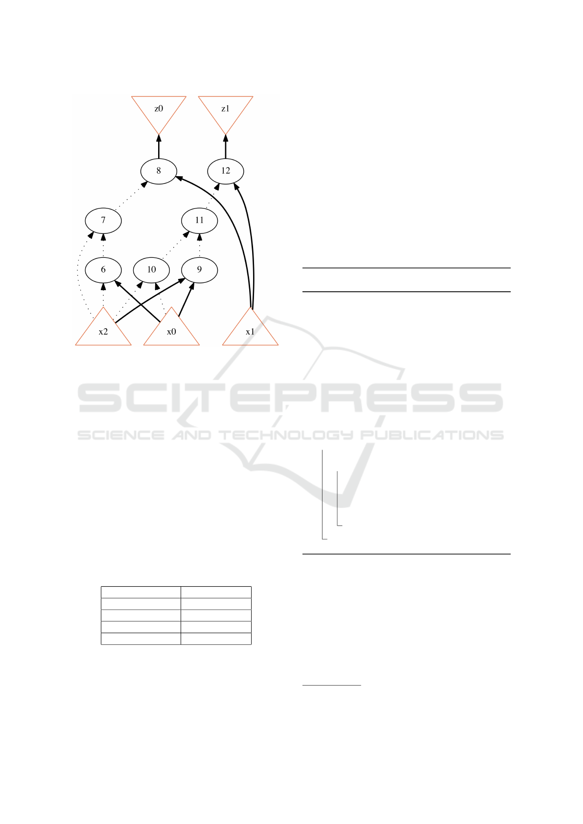
Figure 1: C

Logical Network.

Boolean functions that can be described by a Look-

up-table (LUT). An LUT contains a set of input/out-

put Boolean vectors describing the circuit behavior.

As an example, consider the circuit C

described

by the LUT shown in Table 1; C

is represented by a

logic network in Figure 1. Note that the logic network

has 14 gates, 3 primary inputs ({x0,x1, x2}) and 2 pri-

mary outputs ({z0, z1}). Furthermore, only AND and

NOT gates (the circuit is designed as an And-Inverter

Graph or AIG) are present in the network; AND gates

are represented by the circles while the NOT gates

are depicted as dashed lines. There exist a number

of methods to synthesize a circuit from a system of

Boolean functions or LUTs which can be only par-

tially speciﬁed. In this paper, we do not focus on such

methods, however, in order to perform such synthesis,

we use ABC, a tool for logic synthesis and veriﬁca-

tion (Brayton and Mishchenko, 2010).

Table 1: C

LUT.

x0,x1, x2 (inputs) z0,z1 (outputs)

010 01

011 10

111 11

110 10

A Field Programmable Gate Array (FPGA) is

a device which can be reconﬁgured (programmed)

(Brown et al., 2012) by users, usually through a hard-

ware description language such as Verilog (IEEE,

2017). An FPGA circuit has an array of conﬁg-

urable logic blocks and respective communication

channels

, to achieve the proper reconﬁguration. An

FPGA circuit can be seen as a re-conﬁgurable (com-

binational) circuit.

2.2.1 Using Digital Circuits for Prediction

As shown in (Kushik and Yevtushenko, 2015), there

exists an algorithm that synthesizes a digital circuit

that can be used to ‘predict’ values based on a train-

ing data set. A slight modiﬁcation of this algorithm

is shown in Algorithm 1. For the unknown param-

eter values the circuit can be synthesized based on

the smallest distance to the vectors included in the

LUT (Kushik et al., 2016).

Algorithm 1: Algorithm to synthesize a logic circuit

for prediction.

Input : D

m×n

, a data (training) set, and a

vector of its expected outputs O

Output: C, a logic circuit

1. Determine the number of primary inputs and

primary outputs of C:

The number of primary inputs equals

∑

i=1

dlog

(max(D

) + 1)e, where max is a

function that calculates the maximum value

for a vector (for the i-th parameter); likewise,

the number of primary outputs equals

dlog

(max(O) + 1)e

2. Derive an LUT L from D and O

2.1. Set L to

2.2. for i = 1,2, .. ., m do

2.2.1. Set I empty

2.2.2. for j = 1,2,...,n do

2.2.2.1. Set I to I.bin(d

i, j

), where .

denotes the concatenation operator

between two Boolean vectors and bin

a function that transforms its input to

binary encoding

2.2.3. Set L to ∪ {I/O

}

3. Synthesize C from L and return C

3 MOTIVATING CASE STUDY

In (L

opez et al., 2017), the authors have showcased

how values of the variables in the source code can re-

ﬂect the trustworthiness of a given application. For

that reason, there is a special interest to assure that

the applications running in constrained and mobile

devices are trustworthy. However, what is trustwor-

thiness in the context of a mobile application for

FPGAs might also contain memory elements as latches,

however, it is not relevant for our approach.

ICSOFT 2018 - 13th International Conference on Software Technologies

520

a constrained device? First, we should emphasize

that a smartphone might not be considered as a con-

strained device of a very restricted class, i.e., c0, c1,

or c2 (Bormann et al., 2014). Likewise, we do not

consider a high-end smartphone as a computation-

ally constrained device neither. Nonetheless, some of

these devices operate with the minimum requirements

and therefore can be considered as computationally

constrained. Moreover, the minimum requirements to

run ‘modern’ versions of mobile operating systems as

Android 4.4 require a minimum of 340MB of RAM

(Google, 2013). Nonetheless, this memory is utilized

for the operating system kernel and user space, and

for that reason, the memory gets consumed with dif-

ferent applications from the user, including memory-

intensive applications as web browsers. As a conse-

quence, this fact leaves fewer resources for checking

the trustworthiness of such applications. Intuitively,

one of the most important aspects which inﬂuences

the trustworthiness of a mobile application is its re-

source utilization. We note that different parameters

might be considered for the resource utilization of a

given mobile application. However, we consider the

following 5 parameters.

1. Heap size: The size of the memory occupied by

the application’s dynamic memory allocation.

2. Stack size: The size of the memory occupied by

the application’s execution thread.

3. CPU usage: The load of the application in per-

centage of utilized CPU(s).

4. Disc usage: The space taken by the application

data.

5. Energy Consumption: The amount of energy con-

sumed by the application.

A very important question that needs to be ad-

dressed is how to estimate the trustworthiness of an

application based on the previously established pa-

rameters. Certainly, if the values of all parameters

are rather big, the application is not trustworthy but,

assuming the application has high disc usage or, low

CPU usage and low heap and stack sizes, perhaps it

means that the application performs some caching and

this is considered trustworthy. What if the trustwor-

thiness of an application is only negatively assessed

when high disc usage is combined with high CPU

usage? Certainly, simple trust management models

are not capable to express complex patterns. How-

ever, the human-cognitive concept of trust can be used

through a self-adaptive model, for example through

the use of a complex machine learning model.

Nevertheless, utilizing such complex machine

learning approach inside a computationally con-

strained device seems rather contradicting. In this pa-

per, we attempt to overcome this complexity through

the replacement of software to hardware solutions.

As shown in Algorithm 1 (Kushik and Yevtushenko,

2015), a digital circuit can be ‘trained’ to produce the

desired result. In the current work, we employ this

technique to predict the trustworthiness of the appli-

cations being executed in the computationally con-

strained devices. We note that this technique seems

suitable given the fact that values in the data set are

small due to its nature, i.e., resource utilization in

a computationally constrained device. Nevertheless,

there exist some limitations in utilizing known strate-

gies for logic synthesis for the binary classiﬁcation

problem. In the next section, we outline these limita-

tions, and provide solutions to them.

4 DIGITAL CIRCUITS AS

SCALABLE MACHINE

LEARNING APPARATUS

The algorithm to synthesize a digital circuit for ‘pre-

diction’ using a data set (Algorithm 1) has one ma-

jor limitation. In fact, the digital circuit implements

a system of Boolean functions F , where |F | is the

number of primary outputs. Moreover, these func-

tions are partially speciﬁed, and the number of train-

ing examples is much smaller than the number of pos-

sible inputs (combinations).

One might think of this problem as the model nat-

urally over-ﬁts to the trained data set. At the same

time, over-deﬁning the behavior of partially speci-

ﬁed functions from F for the tested set is performed

via logic synthesis solutions, and thus the prediction

model is as good as such synthesis can make it. To

better outline the problem, and the proposed solution,

we present the following running example. Assume a

data set D, as shown in Figure 2, with two features,

x1 and x2, where the classes are labeled by o ∈ {0, 1},

the blue x represents a positive (1) class, and the pink

circle represents the negative (0) class.

To synthesize a digital circuit from the data set

D using Algorithm 1, a data transformation is neces-

sary, to only include positive values. To do so, a sim-

ple normalization can be used in this case, by shift-

ing the origin to the minimum point in the feature

space. For example, the point (0,−2) becomes (2,0)

as the minimum point in the feature space is x1 = −2,

and x2 = −2. The circuit C obtained from the data

set D (depicted in Fig. 2) is depicted in Figure 3 (as

an and-inverter graph), where 2-input and gates are

represented by circles, NOT gate is represented by a

dashed line in the connector of the gate to invert, the

Scalable Supervised Machine Learning Apparatus for Computationally Constrained Devices

521

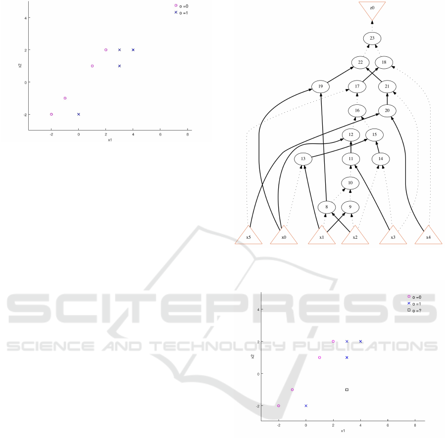
Figure 2: Example data set.

primary inputs are represented in triangles, and the

output is represented as an inverted triangle.

As an example, it can be easily veriﬁed that the

input (0,−2) is correctly predicted as 1 using C with

encoded inputs x1 = 0, x2 = 1, x3 = 0, x4 = 0, x5 = 0,

x6 = 0. The encoding process ﬁrst transforms the in-

put data to the shifted point (2,0), then a binary trans-

formation results in (010000). But, what about the

input (3,−1)? The output of C for the encoded in-

put x1 = 1, x2 = 0, x3 = 1, x4 = 0, x5 = 0, x6 = 1

is 0. One of the possible explanations for this behav-

ior is that the algorithm used to synthesize the circuit

‘considers’ unspeciﬁed patterns as 0. Another possi-

bility is that in order to optimize the number of gates,

a particular gate is chosen which for the speciﬁed pat-

terns behaves as listed but, behaves different for other

patterns; for example, for the patterns (1, 0) and (0,

1) both OR and XOR gates ‘behave’ equally, but not

for (1,1). Indeed, the algorithm used by ABC (Bray-

ton and Mishchenko, 2010), the tool to synthesize the

circuit C (as shown in Fig. 3) assumes that unseen pat-

terns are 0. However, as shown in Figure 4, this un-

speciﬁed input seems to belong to the 1 class. There-

fore, the question arises, how can a circuit which pos-

sesses better generalization of the unseen data be syn-

thesized? Or, in other words, which logic synthesis

approach can be utilized when the criterion of opti-

mality is not a traditional one, such as for example,

the number of gates, the path length from primary

inputs to primary outputs, the surface or circuit pla-

narity, etc. but, the prediction accuracy over the tested

patterns? As mentioned above, for undeﬁned patterns,

the ‘prediction’ circuit can be synthesized based on

the smallest distance to the vectors included in the

LUT.

Figure 3: Digital circuit for ‘predicting’ the class given the

data set D.

Figure 4: Unspeciﬁed data pattern.

4.1 An Inductive Machine Learning

Approach

In the literature, different machine learning mod-

els have been proposed to achieve the classiﬁcation

(Christopher, 2016). Some of these models are widely

adopted. As an example, Support Vector Machines

(SVMs) (Boser et al., 1992) are known to have good

prediction performance regardless of the complexity

and non-linearity of the data. In (L

opez and Maag,

2015), an algorithm to train an SVM with high accu-

racy independent from the data is showcased. For the

example data set D, an SVM trained with the latter

ICSOFT 2018 - 13th International Conference on Software Technologies

522

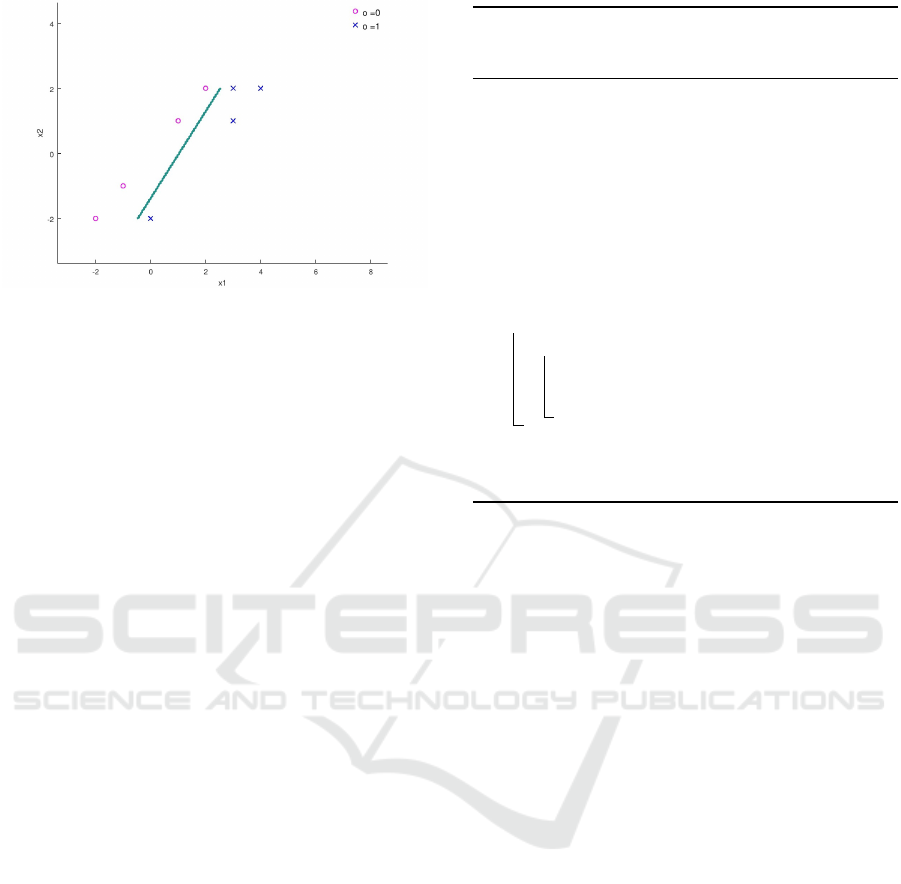
Figure 5: SVM Decision boundary for the dataset D.

mentioned algorithm delivers the decision boundary

as shown in Figure 5.

We propose an inductive approach which ‘learns’

the undeﬁned (unseen) patterns from a model that has

high accuracy and good generalization for prediction.

Generally speaking, the naive algorithm to achieve

that is to train a desired model M (e.g., a SVM), and

use M to predict each of the points of interest to later

add as training examples and to synthesize the cir-

cuit using Algorithm 1. We recall at this point that

under the assumption that the feature space is ‘lim-

ited enough’ this is feasible. However, when dealing

with binary classiﬁcation, this naive algorithm can be

improved by the use of a heuristic. The heuristic is

straightforward, we take advantage of the fact that

both unseen and 0 patterns are considered as 0. For

that reason, we propose that the training set to syn-

thesize the digital circuit only includes patterns which

are 1.

An interesting conclusion after training the circuit

C with the patterns obtained from M is that the cir-

cuit has the same prediction accuracy of M for cer-

tain bounds of the feature space. For example, all the

training examples that appear in D (the running ex-

ample) can be described as a vector of min/max pairs,

e.g., ((−2,−2), (4,2)). Furthermore, a purely com-

binational digital circuit can be implemented in hard-

ware, and this small apparatus can be integrated into a

computationally constrained device; the performance

of such physical prediction chip is extremely high.

Certainly, another option is to use any hardware de-

scription language together with an appropriate dig-

ital circuit simulator inside the computationally con-

strained device. In Algorithm 2, we present an algo-

rithm that designs a digital circuit with the prediction

power of a complex prediction model. An important

remark is that the algorithm works for any prediction

model with a reasonably bounded feature space.

Algorithm 2: Algorithm to synthesize a logic circuit

for prediction using the values of a trained machine

learning model M.

Input : M a trained machine learning model,

and B = (in f ,sup)

,in f , sup ∈ Z, a

vector of n elements representing a

hypercube of the bounded area of

interest for the feature set

Output: C, a logic circuit for prediction

simulating M

0. Set the row index r to 1

1. Set D

as an empty matrix of n columns

2. foreach point p ∈ B (inside the bounds of

interest) do

2.1. if M(p) = 1 then

2.1.1. Add p as the r-th row of the D

matrix

2.1.2. Increment r

3. Use Algorithm 1 to synthesize a circuit C

from D

and 1 (a vector of 1’s of size

m = r − 1), and ﬁnally return C

Discussion. It is important to note that Algorithm 2

synthesizes a digital circuit that predicts as accurate as

the given model M predicts for the given hypercube.

Furthermore, the algorithm can be extended so that

it continues ‘learning’ from M, increasing the size of

the hypercube, for example, until a given timeout or

a space limit are reached. Even though this process

sounds computationally expensive / costly, we must

note that this process is to be done only once. On

the other hand, the algorithm can be easily modiﬁed

for multi-class classiﬁcation, considering the outputs

of M to be included into a vector of expected output

responses to o

and use it to synthesize C in Step 3.

Finally, we note that this approach is valid for any su-

pervised machine learning model. This implies that

many powerful algorithms such as convolutional neu-

ral networks or any other deep learning (Deng et al.,

2014) approach can be employed.

5 DIGITAL CIRCUITS FOR

CASCADE OR HIERARCHICAL

MACHINE LEARNING

CONFIGURATIONS

In the previous section, we have showcased a proce-

dure to synthesize a digital circuit that is capable of

classifying data with the accuracy of a given machine

learning model. In this section, we discuss how given

a set of the previously synthesized digital circuits, bet-

Scalable Supervised Machine Learning Apparatus for Computationally Constrained Devices

523

ter prediction accuracy can be achieved when a cas-

cade composition of such devices is designed.

To better illustrate our approach, we introduce a

sample data set D2 (with expected outputs O), as

shown in Figure 6. It is certainly possible to train

a single self-adaptive model that separates between

the different classes of D

, and furthermore, with

good accuracy. For example, when training an SVM

as suggested in (L

opez and Maag, 2015), the cross-

validation accuracy percentage reaches ∼ 96.67%.

However, as seen in D

, all classes seem to be lin-

early separable, in exception of classes 3 and 4. Fur-

thermore, if merging classes 3 and 4 as the virtual

class 6 all classes are linearly separable, as shown in

Figure 7; when creating a classiﬁer for the newly cre-

ated data set, a 100% cross-validation accuracy can

be obtained. Likewise, if considering only the 3 and 4

classes in D

a classiﬁer with a 100% cross-validation

accuracy can be trained (as shown in Figure 8).

Figure 6: Sample Multi-class data set (D

Figure 7: Classiﬁcation for D

with merged non-linearly

separable classes.

Both classiﬁers shown in Figures 7 and 8 can

be implemented in two different logic circuits LC1

and LC2 respectively. Nevertheless, how to combine

both prediction circuits? One possible solution is to

use LC1 to classify the data in exception whenever

Figure 8: Classiﬁcation for classes 3 and 4 of D

LC1 outputs the class number 6 (LC2 ‘knows’ bet-

ter); when the output class is 6 then use LC2 to de-

cide on the proper class. In the literature, such cas-

cade conﬁgurations have been successfully utilized to

accurately predict overlapping classes (see, for exam-

ple (Tarando et al., 2017)). To achieve the desired

cascade conﬁguration, we propose the use of tradi-

tional data selection circuits known as multiplexers.

A multiplexer is a logic circuit that based on the se-

lector chooses from different input signals and repli-

cates the selected input signal to its (single) output.

As an example, consider a binary (two inputs) mul-

tiplexer with 3 primary inputs as shown in Figure 9;

the multiplexer sends to its output the values at the

input values (x1,x2,x3) if the selector input equals 0

and respectively sends (y1,y2, y3) if the selector input

equals 1.

Figure 9: binary 3-input multiplexer.

The resulting conﬁguration is shown in Figure 10.

Note that the circuit LC3 is a very simple circuit im-

plementing the following Boolean function LC3(x1,

x2,x3) = x1 ∧ x2 ∧ x3, which outputs 1 whenever the

output of LC1 is 6 (binary 110). The circuit shown

in Figure 10 has a 100% cross-validation accuracy for

all classes in D

An algorithm to construct ‘cascade’ compositions

of logic circuits and a multiplexer is shown in Algo-

rithm 3. As an example, the algorithm executed with

inputs LC1, LC2, 6 respectively, produces the circuit

shown in Figure 10 where Mx (BinMux) produces

outputs of the LC1 (the principal classiﬁer) when the

selector (LC3) input is 0 while producing outputs of

ICSOFT 2018 - 13th International Conference on Software Technologies

524

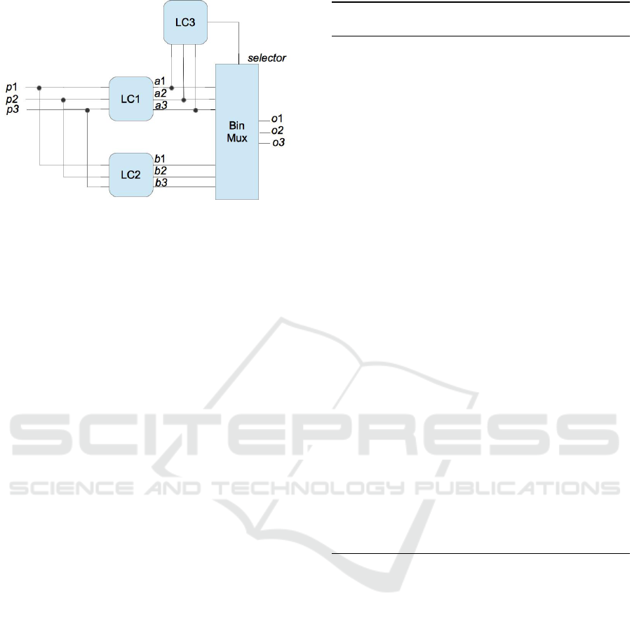
Figure 10: Cascade classiﬁcation architecture using digital

circuits.

LC2 (the secondary classiﬁer) otherwise.

Note that in Algorithm 3 we assume, for the sake

of simplicity that the primary number of inputs and

outputs of LC1 and LC2 which represent the principal

and secondary classiﬁers coincide. Further, it is im-

portant to note that the predictions relied on the sec-

ondary classiﬁer can be present at different regions of

the primary classiﬁer. Moreover, our approach can be

easily extended to consider more than two classiﬁers,

however, these extensions are out of the scope of this

paper, and left for future work. Finally, it is impor-

tant to highlight that creating a composition of devices

can be motivated due to different reasons, other than

achieving a better prediction accuracy. One of exam-

ples in this case is the pre-existence of certain devices

trained for speciﬁc data patterns.

6 PRELIMINARY

EXPERIMENTAL RESULTS

To validate our approach, an experimental evaluation

was conducted to compare how fast and scalable can

be a trained complex model as an SVM or an Artiﬁ-

cial Neural Network (ANN) against a digital circuit

constructed from the complex model. As machine

learning implementations vary, as well as the possi-

bilities to implement a logic circuit, different exper-

iments, comparing different apparatus to implement

them were performed. Moreover, the experiments

were conducted using different experimental setups,

to further validate the consistency of our experiments

across various conﬁgurations. We showcase those ex-

periments and provide their context in the following

subsections.

Algorithm 3: Algorithm to synthesize a cascade com-

position of logic circuits for prediction.

Input : P, a principal prediction classiﬁer as a

digital circuit; S, a secondary

prediction classiﬁer as a digital

circuit; o, a “virtual class” for the

classiﬁer P to be replaced with the

predictions of the classiﬁer S

Output: C, a cascade logic circuit

1. Set o

to the binary representation of o, the

length of o

must be equal to the number of

primary outputs of P; using o

/1 synthesize V ,

a selector logic circuit

2. Set the number of primary inputs of C to the

number of primary inputs of P; likewise, set

the number of primary outputs of C to the

number of primary outputs of P

3. Connect the primary inputs of C to those of

P and S

4. Derive a binary multiplexer Mx with the two

input signals corresponding to the primary

outputs of P and S respectively, and a single

input for the signal selection; the number of

primary outputs of Mx equals the number of

primary outputs of P

5. Fork the primary outputs of P and connect

them to the primary inputs of V and to the ﬁrst

input signal of Mx

6. Connect the output of V to the selector input

of Mx

7. Connect the primary outputs of S to the

second input signal of Mx

8. return C where primary outputs of C are

primary outputs of Mx

6.1 Well-known Machine Learning

Implementation Environment vs. a

Simulated Digital Circuit

The motivation behind these experiments is to show-

case that after a machine learning model has been

obtained in well-known mathematical programming

languages, it is comparatively slower than a simula-

tion of its digital circuit equivalent. We chose to com-

pare both approaches as they can be (arguably) con-

sidered to be the slowest of both domains.

The experiments were conducted in a virtual ma-

chine running CentOS 6.9 with 2 Intel(R) Core(TM)

i5-2415M CPU @ 2.30GHz processors, 3GB of

RAM, executed under a VirtualBox Version 5.1.30

r118389 for Mac OS X 10.13.1. Using the exam-

ple data set D from Section 4, the matrix represent-

Scalable Supervised Machine Learning Apparatus for Computationally Constrained Devices

525

ing the area (hypercube in the general case) of inter-

est as B = ((−2, −2),(4,2)), and a trained SVM M

as inputs for Algorithm 2, the obtained circuit was

simulated to predict the unknown pattern (3,−1) (as

shown in Fig. 4).

The ABC tool version 1.01 was used for the sim-

ulation of the pattern (using the sim command). As

the simulation time was so little and ABC does not

provide a precise way to measure the time to simulate

a single pattern, the pattern 101001 (after the shifting

and binary encoding) was simulated 10000 times. The

resulting time for the simulation was 0.02s. There-

fore, on average, each simulation took ∼ 2 ∗ 10

−6

When using GNU Octave version 3.4.3 with LibSVM

version 3.22, the time for predicting the same pattern

was 9.5∗10

−4

s. Therefore, the performance obtained

by using the presented approach was 424 times faster

than the prediction using a complex model (and pro-

gramming language). Nonetheless, thorough experi-

mental investigation is needed to obtain a more pre-

cise value of the speed up.

6.2 Optimized Machine Learning

Libraries / Implementations vs.

Optimized Digital Circuit

Simulation

The motivation behind these experiments is to show

that optimized implementations for machine learning

models are still comparatively slower than a digital

circuit implemented in software. Furthermore, the ex-

periments show that given the nature of a digital cir-

cuit representation, the prediction time does not de-

pend on the complexity of the underlying model (the

model M used to synthesize the circuit).

The experiments were conducted in a computer

with the following features: an Intel(R) Cor(TM) i5-

3210M CPU @ 2.5 GHz, with 8 GB of RAM, running

the operating system GNU/Linux Ubuntu 14.04 (ker-

nel 4.4.0-119-generic).

The Fast Artiﬁcial Neural Network li-

brary (FANN) (Nissen, 2003) allows rapid load

and execution of a trained ANN. Furthermore,

when using FANN through a compiled program, the

computation time for predicting the class / value

for a given input vector is short. To ‘optimize’ a

digital circuit simulation, we also provide a compiled

version of a digital circuit. For these experiments,

after obtaining the desired circuit from the original

(FANN provided) neural network, we used the

ABC (Brayton and Mishchenko, 2010) tool to output

the circuit into the Verilog (IEEE, 2017) format. As

the syntax of Verilog highly resembles the C syntax,

we manually translated these simple speciﬁcations

into C programs and compiled them

. To compare

the approaches, different ANNs were generated, from

a randomly generated data set. Note that the ANNs

were generated with different numbers of hidden

nodes. Each ANN was (i) generated with the FANN

library, and (ii) converted to a compiled program

simulating the corresponding digital circuit. The time

taken to process an input vector is shown in Table 2.

Table 2: Speed-up results for the simulation of optimized

digital circuits.

Hidden

nodes

FANN avg.

time (ms)

Circuit avg.

time (ms)

Circuit

Speed-up

10 1.8917761 1.5471885 1.22

20 2.024755 1.5657246 1.29

30 2.1441107 1.5544505 1.38

40 2.2387445 1.6087804 1.39

50 2.2489767 1.5748608 1.43

60 2.4201026 1.5526805 1.56

70 2.4620724 1.5614781 1.58

80 2.6246381 1.5584424 1.68

90 2.7182679 1.5445390 1.76

100 2.7970853 1.4505086 1.93

It is important to note that due to inherent char-

acteristics of the ANN model different conﬁgurations

require longer time; for example, an ANN with more

hidden nodes (neurons) in the network. As deep

learning (Deng et al., 2014) is increasingly gaining

attention, the number of inputs, and hidden layers

in neural networks is expected to be considerably

large thus, signiﬁcantly affecting the prediction per-

formance. On the other hand, as Table 2 shows the

prediction time for a digital circuit is stable. There-

fore, the speed-up obtained by the digital circuit rep-

resentation consistently increases as the model gets

more complex.

6.3 Field-programmable Gate Array

Implementations

We would like now to showcase a ‘close-to-real’ per-

formance evaluation of what digital circuits used for

classiﬁcation / prediction can provide. Further, it is

expected that in order to provide a possibility to reﬁne

the prediction model for computationally constrained

devices, FPGA circuits can be employed.

The experiments were preformed by compil-

ing Verilog ﬁles obtained from synthesizing digi-

tal circuits from machine learning models as shown

To verify the correct translation, the original data set

used to synthesize the ANN was used to compare the digital

circuit program against the trained ANN.

ICSOFT 2018 - 13th International Conference on Software Technologies

526

in Algorithm 2, to the Cyclone V GX FPGA

(5cgxfc5c6f27c7n (Altera Products, 2014)). To mea-

sure the time the FPGA takes to process an input, the

propagation delay was used, i.e., the time a logic sig-

nal takes from the primary input to the primary output

was measured.

As expected, the average propagation time was

largely smaller than any software-based response

time. On average, the propagation time for an FPGA

circuit which implements the behavior of a complex

machine learning model was 11,543 nanoseconds.

The speed-up is therefore, in the order of ten thou-

sand times. Arguably, a digital circuit assembled for

the particular purpose might have better performance,

however, as FPGA circuits seem to be better suited for

the prediction task in computationally constrained de-

vices, we focused on them. Moreover, the real time to

communicate with the prediction circuit was not taken

into account in the current experiments and further

work implementing the approach on real constrained

devices is necessary to accurately evaluate the time

speed-up. In order to validate the cascade composi-

tion approach, a digital circuit was synthesized and

programmed into an FPGA circuit. As expected, the

circuit possesses the prediction accuracy of the ma-

chine learning cascade composition and the inexpen-

sive features of a digital circuit.

6.4 Discussion

We note that the complexity issues for the proposed

approach (Section 4) impose a number of limitations

on its applicability. In fact, the main complexity ‘is

hidden’ in Steps 2 of both Algorithms 1 and 2. Indeed,

the number of iterations to build an LUT for the logic

circuit derivation dramatically affects the scalability

of the proposed approach. When the number of rows

m in the data set depends in a polynomial way on the

number of signiﬁcant trust parameters, the complex-

ity of the derivation of the cascade logic circuit can be

also approximated with a proper polynom. However,

on the other hand, the bigger is m the more precise

is the prediction. Performing the preliminary experi-

ments allowed us to draw some conclusions about this

precision / scalability trade-off.

Evidently, in this case, the size of the hyper-cube

is a limitation of the approach. However, computing

the expected values in the hyper-cube until a given

time or space limit is a common heuristic. The ap-

proach is applicable for smaller hyper-cubes of inter-

est as in the motivating case study presented in Sec-

tion 3. We conclude that a mobile application running

in a constrained device should use at most few units

in MB for heap and stack sizes, and for disc utiliza-

tion; it should also use few units of CPU percentage;

likewise, few units of micro-amperes for the energy

consumption. For that reason, the number of patterns

labeled as trustworthy is expected to be small, and the

obtained digital circuit to predict the trustworthiness

of a mobile application is expected to have a relatively

small number of inputs. Therefore, even if the num-

ber of rows m grows exponentially w.r.t. the number

of trust parameters, the power of the exponent can still

be limited by a feasible constant. Nonetheless, we

note that further experimental evaluation is necessary

to carefully estimate when the approach is applicable

and / or preferable.

7 CONCLUSION

In this paper, we presented an approach to synthesize

digital circuits that reproduce the behavior of complex

machine learning algorithms. Such digital devices

can be used as scalable apparatus for complex classiﬁ-

cation / prediction in computationally constrained de-

vices. We note that the proposed approach is generic

and can be applied for implementing any (semi-) su-

pervised machine learning technique as the corre-

sponding hardware device. In this paper, for exam-

ple, we focused on neural networks and support vec-

tor machines utilized for this purpose. We show-

cased later on how cascade compositions for machine

learning-based devices can be achieved through using

a digital multiplexer. Such compositions have high

accuracy prediction level, and at the same time they

are not resource consuming (computationally inex-

pensive). Preliminary experimental results show the

applicability and scalability of the proposed approach.

We also notice that when using an appropriate

multiplexer, the proposed approach can be applied for

a cascade composition of two machine learning / self-

adaptive models (Kushik and Yevtushenko, 2015) if

subsets of the data set for effective prediction are

known for each circuit. However, a circuit for such

multiplexer is known to be much simpler than those

for digital circuits and can be not taken into account

when evaluating the processing time and consumed

resources.

As mentioned above, experimental results are

rather preliminary and we therefore plan to perform

large-scale experiments in real environments to fur-

ther validate the applicability and limitations of the

proposed approach. On the other hand, we would like

to try different (machine-learning-based) digital cir-

cuit compositions to try to estimate the prediction ac-

curacy for each of such compositions. Furthermore,

an interesting perspective is to study the use of digital

Scalable Supervised Machine Learning Apparatus for Computationally Constrained Devices

527

circuits for unsupervised and reinforcement learning.

ACKNOWLEDGEMENTS

The authors would like to thank Prof. Roland Jiang,

and his group at National Taiwan University for the

organized seminars and fruitful discussions that par-

tially inspired this research. The results in this work

were partially funded by the Russian Science Foun-

dation (RSF), project # 16-49-03012.

REFERENCES

Altera Products, A. C. (2014). Altera mature devices.

https://www.altera.com/products/fpga/overview.html.

Bormann, C., Ersue, M., and Keranen, A. (2014). IETF

RFC 7228.

Boser, B. E., Guyon, I. M., and Vapnik, V. N. (1992). A

training algorithm for optimal margin classiﬁers. In

Proceedings of the Fifth Annual Workshop on Compu-

tational Learning Theory, COLT ’92, pages 144–152,

New York, NY, USA. ACM.

Brayton, R. and Mishchenko, A. (2010). Abc: An aca-

demic industrial-strength veriﬁcation tool. In Touili,

T., Cook, B., and Jackson, P., editors, Computer

Aided Veriﬁcation, pages 24–40, Berlin, Heidelberg.

Springer Berlin Heidelberg.

Brown, S. D., Francis, R. J., Rose, J., and Vranesic, Z. G.

(2012). Field-programmable gate arrays, volume 180.

Springer Science & Business Media.

Christopher, M. B. (2016). PATTERN RECOGNITION

AND MACHINE LEARNING. Springer-Verlag New

York.

Deng, L., Yu, D., et al. (2014). Deep learning: methods

and applications. Foundations and Trends® in Signal

Processing, 7(3–4):197–387.

Google, I. (2013). Android 4.4 compatibility deﬁnition.

https://source.android.com/compatibility/4.4/android-

4.4-cdd.pdf. Last accessed: 2018-04-14.

IEEE (2017). Ieee approved draft standard for

systemverilog–uniﬁed hardware design, speciﬁcation,

and veriﬁcation language. IEEE P1800/D4a, July

2017, pages 1–1317.

Intel, C. (2018). Intel movidius neural compute stick

v2.04.00. https://developer.movidius.com. Last ac-

cessed: 2018-05-05.

Kushik, N. and Yevtushenko, N. (2015). Scalable qoe pre-

diction for service composition. In Proceedings of

the 2nd International Workshop on Emerging Soft-

ware as a Service and Analytics - Volume 1: ESaaSA,

(CLOSER 2015), pages 16–26. INSTICC, SciTePress.

Kushik, N., Yevtushenko, N., and Evtushenko, T. (2016).

Novel machine learning technique for predicting

teaching strategy effectiveness. International Journal

of Information Management.

opez, J., Kushik, N., and Yevtushenko, N. (2017). Proac-

tive trust assessment of systems as services. In

Proceedings of the 12th International Conference on

Evaluation of Novel Approaches to Software Engi-

neering - Volume 1: ENASE,, pages 271–276. IN-

STICC, SciTePress.

opez, J. and Maag, S. (2015). Towards a generic trust

management framework using a machine-learning-

based trust model. In 2015 IEEE Trustcom/Big-

DataSE/ISPA, volume 1, pages 1343–1348.

Nissen, S. (2003). Implementation of a fast artiﬁcial neu-

ral network library (fann). Report, Department of

Computer Science University of Copenhagen (DIKU),

31:29.

Tarando, S. R., Fetita, C. I., and Brillet, P. (2017). Cas-

cade of convolutional neural networks for lung texture

classiﬁcation: overcoming ontological overlapping.

In Medical Imaging 2017: Computer-Aided Diagno-

sis, Orlando, Florida, United States, 11-16 February

2017, page 1013407.

ICSOFT 2018 - 13th International Conference on Software Technologies

528