
Clustering-based Under-sampling for Software Defect Prediction
Moheb M. R. Henein, Doaa M. Shawky and Salwa K. Abd-El-Hafiz
Engineering Mathematics and Physics Department, Faculty of Engineering, Cairo University, Giza, 12613, Egypt
Keywords:
Software Defect Prediction, Under-sampling, Clustering, K-means, Artificial Neural Network.
Abstract:
Detection of software defective modules is important for reducing the time and resources consumed by soft-
ware testing. Software defect data sets usually suffer from imbalance, where the number of defective modules
is fewer than the number of defect-free modules. Imbalanced data sets make the machine learning algorithms
to be biased toward the majority class. Clustering-based under-sampling shows its ability to find good repre-
sentatives of the majority data in different applications. This paper presents an approach for software defect
prediction based on clustering-based under-sampling and Artificial Neural Network (ANN). Firstly, clustering-
based under-sampling is used for selecting a subset of the majority samples, which is then combined with the
minority samples to produce a balanced data set. Secondly, an ANN model is built and trained using the
resulted balanced data set. The used ANN is trained to classify the software modules into defective or defect-
free. In addition, a sensitivity analysis is conducted to choose the number of majority samples that yields the
best performance measures. Results show the high prediction capability for the detection of defective modules
while maintaining the ability of detecting defect-free modules.
1 INTRODUCTION
The main purpose of software defect prediction (SDP)
is to classify a software module into defective or
defect-free based on some calculated software met-
rics, and without being intensively tested. Hence, it
reduces both the time and resources that are needed
for the testing process before the software release. An
ideal SDP should correctly classify all modules. Typ-
ically, two classification errors may occur; the first
one originates from classifying a defective module as
defect-free, meanwhile the second error results from
classifying a defect-free module as defective. The
first type is more risky as it causes failures to the
software after release. Also, the second type slows
down the process of releasing software, because the
modules classified as defective are subject to test-
ing and maintenance, hence, additional time and re-
sources are consumed. One of the most challenging
problems facing SDP is the data imbalance. Almost
all SDP data sets suffer from high imbalance ratio be-
tween the defect-free and defective modules. Most of
the software modules are defect-free, thus, they rep-
resent the majority class. Meanwhile, the defective
modules represent the minority class. Data imbal-
ance is the main cause of the first type of classifica-
tion errors, due to the weak representation of the mi-
nority class with respect to the majority class. Since
data imbalance leads the classifier to be biased to-
ward the majority class, it is a serious problem that
needs to be considered carefully in the context of
SDP. Previously, different imbalance learning tech-
niques were applied to SDP (Menzies et al., 2008;
Zheng, 2010; Khoshgoftaar et al., 2010; Riquelme
et al., 2008; Kamei et al., 2007). Class imbalance
learning techniques are divided into two main cate-
gories, namely data level and algorithm level (He and
Garcia, 2009). Data level techniques, also known as
preprocessing techniques, are dealing with the skew-
ness of data by over-sampling the minority class or
under-sampling the majority class or hybrid under-
sampling and over-sampling. Algorithm level tech-
niques, on the other hand, emphasize the minority
samples through assigning higher weights compared
to the majority samples in the learning or the clas-
sification processes. In (Wang and Yao, 2013), five
class imbalance learning methods were applied with
two software defect prediction classifiers on NASA
MDP data sets (Chapman et al., 2004). The two soft-
ware defect predictors are Na
¨
ıve Bayes with log fil-
ter (NB), and Random Forest (RF). The five class
imbalance learning methods include random under-
sampling (RUS), balanced random under-sampling
(RUS-bal), threshold-moving (THM), SMOTEBoost
Henein, M., Shawky, D. and Abd-El-Hafiz, S.
Clustering-based Under-sampling for Software Defect Prediction.
DOI: 10.5220/0006911401850193
In Proceedings of the 13th International Conference on Software Technologies (ICSOFT 2018), pages 185-193
ISBN: 978-989-758-320-9
Copyright © 2018 by SCITEPRESS – Science and Technology Publications, Lda. All rights reserved
185

(SMB), and AdaBoost.NC (BNC). RUS and RUS-bal
belong to data-level methods. THM is a cost sen-
sitive classifier belonging to algorithm level. SMB
and BNC are ensemble classifiers. In (Arar and Ayan,
2015), the authors used a cost sensitive ANN, where
traditional error functions (mean square error, least
square error, relative absolute error, etc.) were re-
placed by Normalized Expected Costed of Misclas-
sification (NECM), which is given by (1).
NECM = FPR × P
nd p
+
C
FN
C
FP
× FNR × P
d p
(1)
Where FPR and FNR are the calculated false pos-
itive and false negative rates, respectively, P
nd p
and
P
d p
are the prior percentage of non-defect prone and
defect prone, respectively, and the term
C
FN
C
FP
defines
the ratio between the costs of false negative error
to false positive error. Due to the imbalance prop-
erty, this term controls the trade-off between two
types of accuracy, overall accuracy and positive de-
tection accuracy. The training process of the ANN
adjusts the weights between neurons using Artificial
Bee Colony (ABC) based on the back-propagated
error from NECM equation.In this paper, we apply
the clustering-based approach that was introduced in
(Lin et al., 2017), for under-sampling the majority
samples. The clustering-based under-sampling ap-
proach is based on balancing an imbalanced data set
by reducing the majority class size to the size of
the minority class. Majority data samples are clus-
tered into number of clusters equivalent to the num-
ber of minority data. Then, for each cluster, only
one sample is selected to replace the whole cluster.
Clustering-based under-sampling can efficiently rep-
resent the whole majority data by a selected subset
instead of random under-sampling. Clustering-based
under-sampling combined with different classifiers
showed high prediction ability on different data sets
in different applications, such as breast cancer (Lin
et al., 2017) and bankruptcy prediction (Kim et al.,
2016). In this paper, we apply this promising ap-
proach with a modified strategy for the selection of
majority data subset for balancing the data sets in the
context of SDP. In this strategy, the clusters’ represen-
tatives are selected in an iterative approach in order to
ensure that the sample was selected at most once. The
rest of the paper is organized as follows: Section 2
discusses the proposed approach. Section 3 describes
the evaluation of the proposed approach in detail, in-
cluding the description of the used data sets, perfor-
mance measures, and the conducted experiments. Fi-
nally, conclusion and future work are given in Section
4.
2 PROPOSED APPROACH
The proposed approach for SDP consists of the fol-
lowing steps. In the first step, the analyzed data
sets are balanced using the clustering-based under-
sampling technique. In the second step, an ANN-
based classifier is built. The built ANN model
was constructed with ten nodes in the single hidden
layer. In addition, Log-sigmoidal function is used as
the transfer function for the hidden layer, and soft-
max function as tranfer function for the output layer.
Adam is used for training the ANN (Kingma and
Ba, 2014). Adam is a gradient-based optimization of
stochastic objective functions.
The clustering-based under-sampling was introduced
in (Lin et al., 2017). The procedure is shown in Fig.
1. The imbalanced data set is divided into major-
ity and minority samples. The majority samples are
clustered, where the number of clusters is equal to
the number of minority samples. For each cluster,
the nearest neighbor sample to the cluster center is
chosen to represent the whole cluster. The clusters’
centers are not suitable for representing the cluster,
because they are artificially calculated samples (Lin
et al., 2017). However, the selection of the nearest
neighbor to clusters center might result in selecting
a sample several times due to overlapping between
clusters. Thus, for preventing duplicates, an iterative
approach for the selection of the majority representa-
tives was used by choosing a unique nearest neighbor
sample to each clusters center in each iteration. Fi-
nally, the selected nearest neighbors samples are com-
bined with the minority samples to form a balanced
data set. In this step, K-means is used for clustering.
K-means clustering algorithm is introduced in (Harti-
gan and Wong, 1979). It calculates the distances be-
tween the target data. The samples with minimum
distances between each other are grouped to form a
cluster. Thus, a cluster combines the samples with
similar characteristics.
3 EVALUATION
3.1 Data Sets
NASAs Metrics Data Program Data Repository
(MDP) is considered as a bench-mark for SDP (Chap-
man et al., 2004). Recently, it was used for the evalu-
ation of SDP models such as in (Wang and Yao, 2013;
Arar and Ayan, 2015; Kumudha and Venkatesan,
2016; L
´
opez et al., 2012; Liu et al., 2014; Li et al.,
2016; Jin and Jin, 2015). It contains defect data of dif-
ferent projects implemented using C, C++, and Java.
ICSOFT 2018 - 13th International Conference on Software Technologies
186
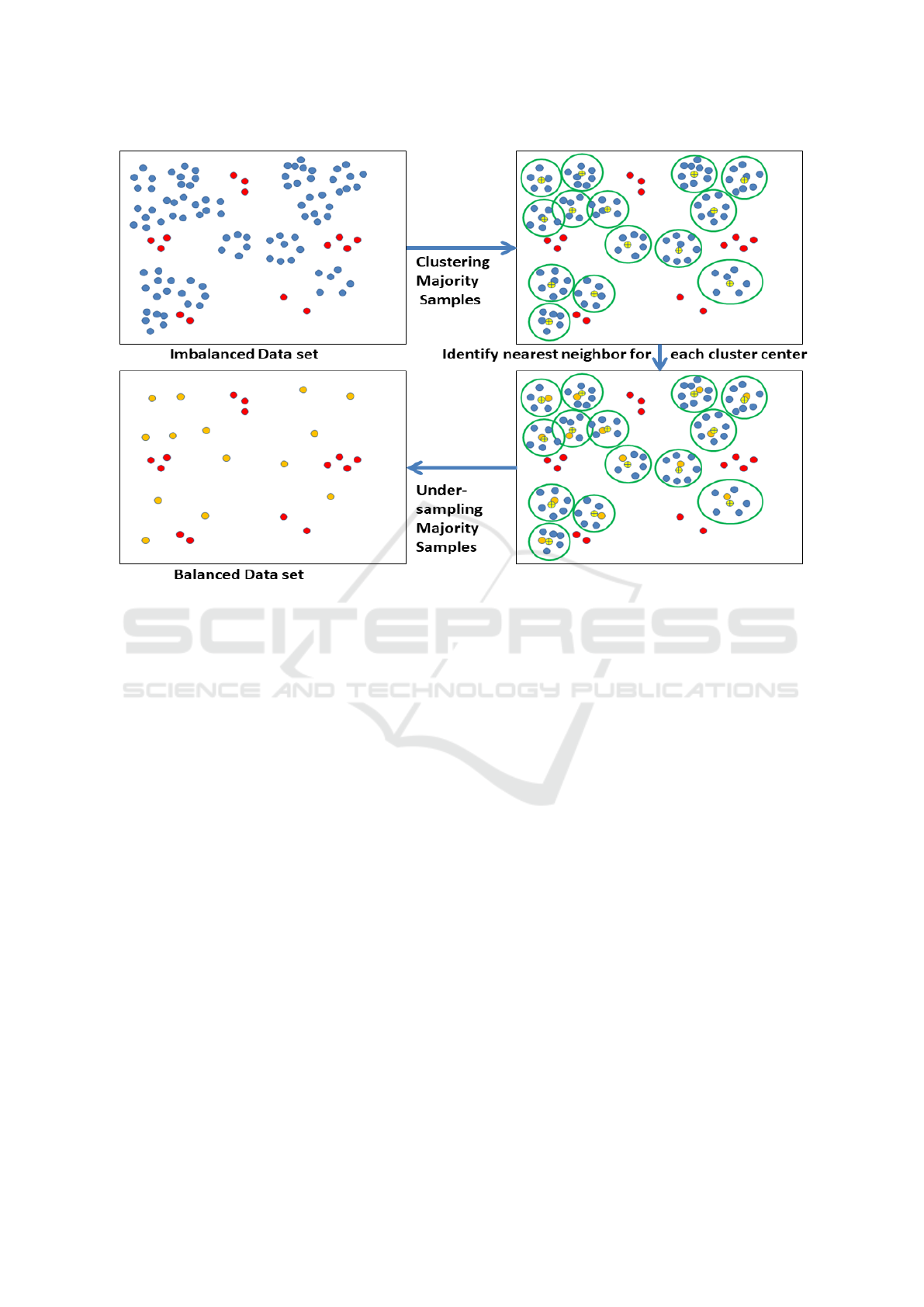
Figure 1: Clustering-based Under-sampling majority samples.
The projects have different sizes and defect ratios.
The software modules are described using different
attributes such as McCabe measures (McCabe, 1976)
and Halstead measures (Halstead, 1977). In this pa-
per, five NASA MPD data sets were selected for the
evaluation of the proposed approach. Since these data
sets were selected by recent similar approaches, we
have applied our proposed approach on them to be
able to conduct a fair comparison. Some descriptions
about the selected data sets from PROMISE reposi-
tory (available at http://promisedata.org/) are shown
in Table 1.
3.1.1 Data Preprocessing
Three preprocessing steps were firstly performed on
the data sets. These steps are recommended by (Gray
et al., 2012; Shepperd et al., 2013) and include the
following:
1. Removing duplicated samples with the same fea-
ture values.
2. Replacing unavailable values by the mean value
of the corresponding feature.
3. Normalizing the feature values. In this paper, a
quantile transformer is used for each feature inde-
pendently by mapping the data to a uniform distri-
bution with values between 0 and 1. This is a non
linear transformation which reduces the impact of
marginal outliers (Pedregosa et al., 2011)
3.2 Performance Measurement
3.2.1 Confusion Matrix
Different performance measurements based on the
confusion matrix are used in the software defect pre-
diction domain for reporting and comparing the re-
sults of different techniques (He and Garcia, 2009;
Wang and Yao, 2013; Arar and Ayan, 2015; Ku-
mudha and Venkatesan, 2016; L
´
opez et al., 2012;
Liu et al., 2014; Li et al., 2016; Jin and Jin, 2015;
Abaei et al., 2015). Table 2 shows a typical confu-
sion matrix where the defect-prone and the defect-free
are considered as positive and negative, respectively.
Confusion matrix for binary classification is formed
by four cells namely, the number of positive modules
truly classified (T P), the number of positive modules
falsely classified (FP), the number of negative mod-
ules falsely classified (FN), and the number of neg-
ative modules truly classified (T N). The following
measurements are calculated based on the elements
of the confusion matrix.
• Overall Accuracy
Accuracy measures the ratio of the truly classified
samples to the total number of samples as given by
Clustering-based Under-sampling for Software Defect Prediction
187

Table 1: NASA MDP data sets description.
Data Description Language Number of Percentage of
set Modules defective modules
CM1 Spacecraft instrument C 498 9.83
KC2 Storage management C++ 522 20.49
for ground data
PC1 Flight software C++ 1109 6.94
for earth
orbiting satellite
KC1 Storage management C++ 2109 15
for ground data
JM1 Real-time predictive C 10885 21.4
ground system
Table 2: Confusion Matrix.
`
`
`
`
`
`
`
`
`
`
`
`
Predicted
Actual
Defect-Prone Defect-Free
Defect-Prone True Positive False Positive
T P FP
Defect-Free False Negative True Negative
FN T N
(2). Accuracy can have values between zero and
one, where accuracy values closer to one mean
that the classifier has a better prediction perfor-
mance.
Accuracy =
T P + T N
T P + FP + T N + FN
(2)
• Probability of Detection (PD) or True Positive
rate(T PR)
PD is the ratio of the actual positive samples truly
classified to the total number of actual positive
samples as given by (3). PD values closer to one
mean that the classifier has a better prediction per-
formance.
PD = T PR =
T P
T P + FN
(3)
• Probability of False Alarm (PF) or false positive
rate (FPR)
PF is the ratio of the actual negative samples
falsely classified to the total number of actual neg-
ative samples as given by (4). PF closer to zero
means that classifier has better prediction perfor-
mance.
PF = FPR =
FP
FP + T N
(4)
• Balance
Balance combines PF and PD into one measure.
It is defined as the Euclidian distance from the real
point (PD, PF) to the ideal point (PF = 0, PD =
1) as given by (5). Balance is expected to be high
for a good predictor.
Balance = 1 −
r
(0 − PF)
2
+ (1 − PD)
2
2
(5)
• F1-measure
F1-measure is calculated based on confusion ma-
trix’ elements as given by (6). F1-measure closer
to one means that classifier has better prediction
performance.
F1 =
2 ∗ (
T P
T P+FP
∗
T P
T P+FN
)
(
T P
T P+FP
+
T P
T P+FN
)
(6)
3.2.2 Receiver Operating Characteristics Curve
(ROC)
ROC curve illustrates the trade-off between the proba-
bility of detection (PD) and the false alarm rates (PF).
It is used in the performance evaluation of a classifier
across all possible decision thresholds. Values of area
under curve (AUC) lie between 0 and 1 (Huang and
Ling, 2005; Bradley, 1997). It is equivalent to the
probability that a randomly chosen sample of the pos-
itive class will have lower estimated probability to be
misclassified than a randomly chosen sample of the
negative class. A good predictor should have a high
AUC value.
3.3 Experiments and Results
Two experiments were performed on the selected data
sets. The first experiment evaluates the performance
ICSOFT 2018 - 13th International Conference on Software Technologies
188
of the proposed balancing approach combined with
ANN. The effect of the number of under-sampling
majority samples was investigated in the second ex-
periment. The experiments were performed using 5-
fold cross validation repeated 10 times for reporting
the mean results, which resulted in 50 runs, in order
to test the robustness of the proposed model by select-
ing different random learning and testing sets for each
run. The experiments were performed using Python,
where scikit-learn library was used for K-means and
performance measures calculation (Pedregosa et al.,
2011). ANN was built using tensorflow with three
layers; namely input layer, hidden layer, and output
layer. Moreover, log-sigmoidal function was used as
transfer function of the hidden layer, that consists of
10 neurons, meanwhile the softmax function is used
as transfer function for the output layer.
3.3.1 Experiment 1
In the first experiment, the data set was balanced by
selecting the number of majority clusters to be equal
to the number of minority samples. Then, each clus-
ter of the majority samples was replaced by a single
sample. The nearest sample to each cluster center was
selected to replace the whole cluster elements. Se-
lection of the clusters’ representatives was performed
in sequence to ensure that the sample was selected
at most once. The selected sample is the nearest
neighbor to the cluster’ center, which should be se-
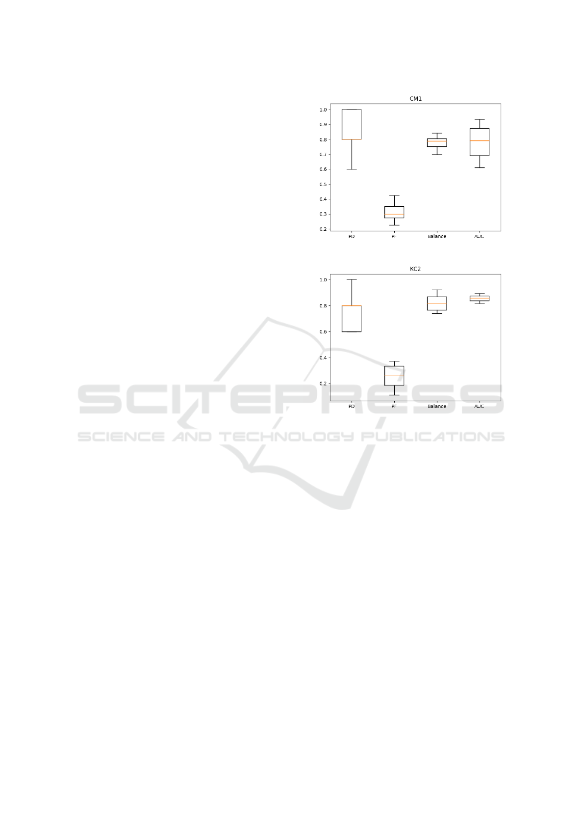
lected only once. Figures 2- 6 show the box plots
of the calculated performance measures for each data
set for the 50 runs. The calculated mean and the
95% confidence interval of performance measures are
given in Table 3. Results show that the proposed
approach is suitable for small scale data sets (CM1,
PC1, and KC2), where the achieved PD values are
greater than 0.7, and PF values are smaller than or
equal to 0.3, also AUC values are around 0.8. Fig-
ures 2-4 show that the proposed approach succeeded
in correctly predicting the defective modules (PD = 1
for some runs). Also, the best achieved PF value for
the small scale data sets is equal to 0.2. Thus, the
results show the ability of the proposed approach to
detect the defective modules while maintaining good
capability for the detection of the defect-free mod-
ules. However, the calculated performance measures
for the relatively large-scale data sets (KC1 and JM1),
are worse than those of the small scale data sets’. Al-
though, the obtained measures for detecting the de-
fective modules are acceptable, since PD values are
greater than or equal to 0.65. The main drawback of
the proposed approach appears in the PF values of the
large data sets, where the PF values are greater than
0.4. The relatively high PF values means that the pro-
Figure 2: CM1 performance measurement box plots.
Figure 3: KC2 performance measurement box plots.
posed approach misclassified some of the defect-free
modules. This can be explained by the loss of infor-
mation about the defect-free modules in the sampling
process, which increases as the size of the data set in-
creases since more samples are removed in this case.
To address this, experiment 2 was conducted.
3.3.2 Experiment 2
In this experiment, a sensitivity study was conducted
by using different numbers of clusters to show the ef-
fect of changing the number of majority class sam-
ples on the overall performance of the proposed sys-
tem. Figures 7-11 show the influence of varying the
number of selected defect-free samples (clusters) on
the performance of the proposed approach using K-
means. As the number of defect free samples in-
creases, while having
the same number of defective samples, the detec-
tion of the defect free modules increases and the de-
tection of the defective modules decreases. Hence,
PD is inversely proportional to the difference be-
tween defect-free and defective samples denoted by
K. However, K is directly proportional to accuracy,
Clustering-based Under-sampling for Software Defect Prediction
189
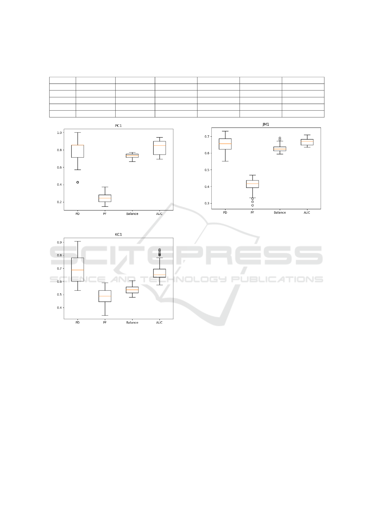
Table 3: Mean values using 95% confidence interval of performance measures achieved by the proposed approach using
K-means for clustering.
Data set PD PF Balance Accuracy AUC F1
CM1 0.836 ± 0.042 0.310 ± 0.014 0.780 ± 0.01 0.706 ± 0.015 0.781 ± 0.028 0.390 ± 0.023
PC1 0.771 ± 0.049 0.249 ± 0.014 0.731 ± 0.0069 0.753 ± 0.014 0.832 ± 0.022 0.318 ± 0.021
KC2 0.754 ± 0.037 0.254 ± 0.021 0.820 ± 0.014 0.748 ± 0.013 0.856 ± 0.0058 0.617 ± 0.019
KC1 0.690 ± 0.028 0.479 ± 0.018 0.540 ± 0.0089 0.566 ± 0.014 0.677 ± 0.02 0.458 ± 0.016
JM1 0.654 ± 0.012 0.406 ± 0.011 0.630 ± 0.0061 0.607 ± 0.0075 0.668 ± 0.0053 0.431 ± 0.0055
Figure 4: PC1 performance measurement box plots.
Figure 5: KC1 performance measurement box plots.
balance, and AUC. Increasing the number of samples
for a class enhances the ability of predicting this class.
Thus, K can be used as a control parameter which
makes SDP model biased toward the detection of de-
fect or defect-free classes. Therefore, based on the
defined costs of misclassification, K can be selected
to minimize the overall cost. Also, a moderate value
of K can be selected in order to have a good accuracy,
balance, and AUC values while having an acceptable
PD value. Thus, performance measures were calcu-
lated at different values of K from −25 to 25 with
step size equals to 5, where the 0 value determines the
balanced data set having the number of selected ma-
jority samples equal to the number of minority sam-
ples. This interval is chosen to test the sensitivity of
the proposed approach to the number of selected ma-
Figure 6: JM1 performance measurement box plots.
jority samples around the balanced data set, and to
prevent the classifier from being biased toward any of
the two classes. As shown in figures 7-11, for each of
the data sets, the best achieved performance measures
appear at different values of K. Table 4 shows the
best achieved performance measures when K is var-
ied from −25 to 25 on each data set. The results show
that higher performance measures can be obtained at
different values of K.
In addition, Table 5 shows the selected values of
K for each data set, where the selected value achieves
low PF while maintaining high PD. Since the AUC
and Balance are calculated in terms of PD and PF,
therefore the selected values of K can be considered
as the best achieving performance. Hence, K can be
determined in the validation process to achieve high
performance measures. In addition, Table 6 shows
the obtained performance using the selected values of
K in comparison with similar approaches. The com-
pared approaches include algorithm level and data
level techniques. The algorithm level techniques in-
clude ABC-ANN (Arar and Ayan, 2015), and DNC
(Wang and Yao, 2013), meanwhile the used data level
techniques are Random Under Sampling (RUS) and
RUS-bal (Wang and Yao, 2013) . The best result
for each measure is highlighted in bold. As shown
in the table, the proposed approach outperformed the
sampling approaches (RUS and RUS-bal). Also, the
results of the performance measures are comparable
to the cost sensitive learning approaches (ABC-ANN
and DNC). ABC-ANN achieved the best PD in four
ICSOFT 2018 - 13th International Conference on Software Technologies
190
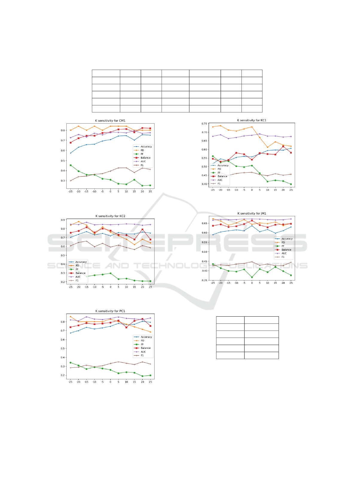
Table 4: Mean values of the best achieved performance measures for different values of K.
Data set PD PF Balance Accuracy AUC F1
CM1 0.84 0.25 0.823 0.755 0.795 0.427
PC1 0.857 0.188 0.832 0.804 0.854 0.349
KC2 0.84 0.207 0.817 0.757 0.854 0.659
KC1 0.84 0.25 0.617 0.606 0.689 0.467
JM1 0.672 0.376 0.823 0.636 0.672 0.444
Figure 7: Performance measurement for different values for
k for CM1.
Figure 8: Performance measurement for different values for
k for KC2.
Figure 9: Performance measurement for different values for
k for PC1.
out of the five data sets, but it gave the worst PF
in the five data sets. This contradiction might be
caused by the greediness of ABC-ANN in predicting
the defective modules, even if it affects the predic-
Figure 10: Performance measurement for different values
for k for KC1.
Figure 11: Performance measurement for different values
for k for JM1.
Table 5: Selected K values for data sets.
Data set Selected K
CM1 10
PC1 5
KC2 0
KC1 20
JM1 0
tion of the defect-free modules. Therefore, the pro-
posed approach outperformed ABC-ANN in Balance
and AUC measures, that are calculated based on PD
and PF measures. Moreover, the proposed approach
achieved better results on small scale data sets (CM1,
PC1, and KC2). Although the results on large scale
data sets (KC1 and JM1) are worse, the results are
comparable to the best performing techniques.
Clustering-based Under-sampling for Software Defect Prediction
191

Table 6: Performance measures of the proposed model versus the state of the art models on NASA data sets.
PD
NASA Data set ABC-ANN RUS DNC RUS-bal Proposed Approach
CM1 0.75 NA
a
0.590 NA 0.84
PC1 0.89 NA 0.570 NA 0.8
KC2 0.79 NA 0.771 NA 0.754
KC1 0.79 NA 0.710 NA 0.625
JM1 0.71 NA 0.660 NA 0.625
PF
NASA Data set ABC-ANN RUS DNC RUS-bal Proposed Approach
CM1 0.33 NA 0.226 NA 0.265
PC1 0.37 NA 0.107 NA 0.22
KC2 0.21 NA 0.216 NA 0.22
KC1 0.33 NA 0.241 NA 0.415
JM1 0.41 NA 0.314 NA 0.415
Balance
NASA Data set ABC-ANN RUS DNC RUS-bal Proposed Approach
CM1 0.71 0.526 0.577 0.577 0.809
PC1 0.73 0.636 0.682 0.688 0.813
KC2 0.79 0.705 0.777 0.709 0.748
KC1 0.72 0.659 0.733 0.677 0.617
JM1 0.64 0.646 0.241 0.642 0.607
Accuracy
NASA Data set ABC-ANN RUS DNC RUS-bal Proposed Approach
CM1 0.68 NA NA NA 0.747
PC1 0.65 NA NA NA 0.782
KC2 0.79 NA NA NA 0.748
KC1 0.69 NA NA NA 0.6
JM1 0.61 NA NA NA 0.607
AUC
NASA Data set ABC-ANN RUS DNC RUS-bal Proposed Approach
CM1 0.77 0.622 0.787 0.622 0.774
PC1 0.82 0.726 0.866 0.739 0.829
KC2 0.85 0.730 0.828 0.726 0.856
KC1 0.80 0.710 0.818 0.713 0.672
JM1 0.71 0.665 0.766 0.658 0.668
a
Not Available.
4 CONCLUSION AND FUTURE
WORK
In this paper, an approach for SDP after balancing
the ratio of defective to non-defective modules is pre-
sented. The balancing is performed using clustering-
based under-sampling on the defect-free modules.
The proposed model improves the detection of the de-
fective modules without affecting the ability to detect
the defect-free modules, which is shown by the high
achieved PD results. In addition, the PF and accu-
racy were improved which means that the detection of
the defect-free modules is also improved. This proves
that clustering-based under-sampling is a good tech-
nique for the selection of a well-representative sub-
set of the majority data for SDP models. As a fu-
ture work, we will apply data samples filtering for re-
moving noisy samples, especially for the large scale
data sets. Also, different clustering and learning algo-
rithms will be investigated.
REFERENCES
Abaei, G., Selamat, A., and Fujita, H. (2015). An
empirical study based on semi-supervised hybrid
ICSOFT 2018 - 13th International Conference on Software Technologies
192

self-organizing map for software fault prediction.
Knowledge-Based Systems, 74:28–39.
Arar,
¨
O. F. and Ayan, K. (2015). Software defect predic-
tion using cost-sensitive neural network. Applied Soft
Computing, 33:263–277.
Bradley, A. P. (1997). The use of the area under the
roc curve in the evaluation of machine learning algo-
rithms. Pattern recognition, 30(7):1145–1159.
Chapman, M., Callis, P., and Jackson, W. (2004). Metrics
data program. NASA IV and V Facility, http://mdp. ivv.
nasa. gov.
Gray, D., Bowes, D., Davey, N., Sun, Y., and Christianson,
B. (2012). Reflections on the nasa mdp data sets. IET
software, 6(6):549–558.
Halstead, M. H. (1977). Elements of software science, vol-
ume 7. Elsevier New York.
Hartigan, J. A. and Wong, M. A. (1979). Algorithm as
136: A k-means clustering algorithm. Journal of the
Royal Statistical Society. Series C (Applied Statistics),
28(1):100–108.
He, H. and Garcia, E. A. (2009). Learning from imbalanced
data. IEEE Transactions on knowledge and data engi-
neering, 21(9):1263–1284.
Huang, J. and Ling, C. X. (2005). Using auc and accuracy
in evaluating learning algorithms. IEEE Transactions
on knowledge and Data Engineering, 17(3):299–310.
Jin, C. and Jin, S.-W. (2015). Prediction approach of soft-
ware fault-proneness based on hybrid artificial neu-
ral network and quantum particle swarm optimization.
Applied Soft Computing, 35:717–725.
Kamei, Y., Monden, A., Matsumoto, S., Kakimoto, T., and
Matsumoto, K.-i. (2007). The effects of over and
under sampling on fault-prone module detection. In
Empirical Software Engineering and Measurement,
2007. ESEM 2007. First International Symposium on,
pages 196–204. IEEE.
Khoshgoftaar, T. M., Gao, K., and Seliya, N. (2010). At-
tribute selection and imbalanced data: Problems in
software defect prediction. In Tools with Artificial
Intelligence (ICTAI), 2010 22nd IEEE International
Conference on, volume 1, pages 137–144. IEEE.
Kim, H.-J., Jo, N.-O., and Shin, K.-S. (2016). Optimiza-
tion of cluster-based evolutionary undersampling for
the artificial neural networks in corporate bankruptcy
prediction. Expert Systems with Applications, 59:226–
234.
Kingma, D. P. and Ba, J. (2014). Adam: A
method for stochastic optimization. arXiv preprint
arXiv:1412.6980.
Kumudha, P. and Venkatesan, R. (2016). Cost-sensitive ra-
dial basis function neural network classifier for soft-
ware defect prediction. The Scientific World Journal,
2016.
Li, W., Huang, Z., and Li, Q. (2016). Three-way decisions
based software defect prediction. Knowledge-Based
Systems, 91:263–274.
Lin, W.-C., Tsai, C.-F., Hu, Y.-H., and Jhang, J.-S. (2017).
Clustering-based undersampling in class-imbalanced
data. Information Sciences, 409:17–26.
Liu, M., Miao, L., and Zhang, D. (2014). Two-stage cost-
sensitive learning for software defect prediction. IEEE
Transactions on Reliability, 63(2):676–686.
L
´
opez, V., Fern
´
andez, A., Moreno-Torres, J. G., and Her-
rera, F. (2012). Analysis of preprocessing vs. cost-
sensitive learning for imbalanced classification. open
problems on intrinsic data characteristics. Expert Sys-
tems with Applications, 39(7):6585–6608.
McCabe, T. J. (1976). A complexity measure. IEEE Trans-
actions on software Engineering, (4):308–320.
Menzies, T., Turhan, B., Bener, A., Gay, G., Cukic, B., and
Jiang, Y. (2008). Implications of ceiling effects in de-
fect predictors. In Proceedings of the 4th international
workshop on Predictor models in software engineer-
ing, pages 47–54. ACM.
Pedregosa, F., Varoquaux, G., Gramfort, A., Michel, V.,
Thirion, B., Grisel, O., Blondel, M., Prettenhofer,
P., Weiss, R., Dubourg, V., Vanderplas, J., Passos,
A., Cournapeau, D., Brucher, M., Perrot, M., and
Duchesnay, E. (2011). Scikit-learn: Machine learning
in Python. Journal of Machine Learning Research,
12:2825–2830.
Riquelme, J., Ruiz, R., Rodr
´
ıguez, D., and Moreno, J.
(2008). Finding defective modules from highly unbal-
anced datasets. Actas de los Talleres de las Jornadas
de Ingenier
´
ıa del Software y Bases de Datos, 2(1):67–
74.
Shepperd, M., Song, Q., Sun, Z., and Mair, C. (2013). Data
quality: Some comments on the nasa software defect
datasets. IEEE Transactions on Software Engineering,
39(9):1208–1215.
Wang, S. and Yao, X. (2013). Using class imbalance learn-
ing for software defect prediction. IEEE Transactions
on Reliability, 62(2):434–443.
Zheng, J. (2010). Cost-sensitive boosting neural networks
for software defect prediction. Expert Systems with
Applications, 37(6):4537–4543.
Clustering-based Under-sampling for Software Defect Prediction
193
