
Energy Efficient Path Planning of Hybrid Fly-Drive Robot (HyFDR)
using A* Algorithm
Amir Sharif, H. M. Lahiru, S. Herath and Hubert Roth
Department of Control Engineering, University of Siegen, Germany
Keywords: HyFDR (Hybrid Fly-Drive Robot), A* Algorithm, Ground Nodes, Autonomous Navigation, Aerial Nodes.
Abstract: Hovering flight is agile and energy expansive, but driving on ground is slow and energy efficient method of
locomotion. To get the benefits of these two methods of locomotion, we combined them in a single platform
named as HyFDR. It is a Quadcopter with powered wheels, it can fly in air and drive on ground.
Autonomous navigation of HyFDR creates new challenges in the field of path planning. The goal is to
simulate the navigation of HyFDR with minimum energy consumption using A* algorithm. Depending
upon the terrain, obstacles, energy constraints, and desired flight time, HyFDR can autonomously switch
between flight mode, drive mode and hybrid mode. We showed that in some cases HyFDR is energy
efficient than Quadcopter.
1 INTRODUCTION
Quadcopters have six degrees of freedom, which
makes obstacle avoidance easy and their locomotion
fast. Beside air drag, they require a continuous
upward force against gravity to hover in air. This
makes hovering flight energy expansive (Dietrich,
2017). Vehicles that drive on ground with wheels,
require no hovering force against gravity, which
makes them less energy expansive. During driving
on ground, most of energy is consumed to overcome
friction forces and air drag. Driving on ground with
wheels has limited degrees of freedom, which makes
the locomotion slow and difficult to avoid obstacles
in the path.
To get the agility and energy efficiency in a
single platform, four powered wheels were added to
a simulation model of Quadcopter. This hybrid
platform is named as HyFDR. It can fly in air like a
normal Quadcopter and drive on ground. Addition of
driving mechanism to a quadcopter increases its
weight, but if the path has sufficient driving
opportunities then this increase in weight can be
compensated by using driving mode more
frequently.
The autonomous navigation of HyFDR created
new challenges in the field of locomotion mode
selection, obstacle avoidance, energy efficient path
planning, and travel time. Many algorithms are
proposed by researchers for the path planning of
mobile robots with single mode of locomotion, but
not much research has been done for the path
planning of mobile robots with dual mode of
locomotion.
A virtual world in Gazebo simulator was created.
Three different test cases were created by addition of
obstacles at different positions in the virtual world.
A 3D map of the environment was made. The nodes
in the map were divided into four types, movement
cost for each type of node was calculated. A
modified A* algorithm was used to find the path
with least energy consumption. During simulation,
HyFDR followed the path created by A* algorithm,
it autonomously navigated through the environment,
avoiding obstacles, switching between flight mode
and driving mode autonomously and reached the
target. The energy efficiency of HyFDR depends
upon the obstacles in the path and the duration of
driving on ground.
1.1 Related Work
Hybrid mobile robots are made by addition of active
or passive driving mechanism to a flying vehicle.
These hybrid mobile robots can fly in air and drive
on ground. They have better energy efficiency and
agility. A Bio-inspired Morphing Micro Air and
Land Vehicle is a micro aircraft with two wings,
flaps, rudder and a front main rotor for propulsion. It
is capable of locomotion in air and on ground as
Sharif, A., Lahiru, H., Herath, S. and Roth, H.
Energy Efficient Path Planning of Hybrid Fly-Drive Robot (HyFDR) using A* Algorithm.
DOI: 10.5220/0006912602010210
In Proceedings of the 15th International Conference on Informatics in Control, Automation and Robotics (ICINCO 2018) - Volume 2, pages 201-210
ISBN: 978-989-758-321-6
Copyright © 2018 by SCITEPRESS – Science and Technology Publications, Lda. All rights reserved
201
well (Jones, 2006). One of its unique features is its
powered legs for crawling on the ground. A multi
modal flying and walking robot (Daler, 2015) has a
rotor on the front side and its wings are foldable.
During aerial locomotion it acts like an air plane but
during locomotion on ground its foldable wings act
like legs. Flying Monkey robot (Mulgaonkar, 2016)
is a world's smallest Quadrotor with the capability of
flying, walking on the ground and grasping objects.
It has a total weight of 30 grams, a tiny battery but
the combination of flight and walking increases its
mission life.
HyTAQ is a Quadcopter supported inside a cage-
like structure which acts as a passive wheel for
locomotion on ground (Kalantari, 2014). This
combination increases its range as compared to the
flying-only Quadcopters and it also solves the
problems of obstacle avoidance related with wheeled
robots. Quadroller (Page, 2014) is developed by
addition of three pairs of passive skateboard wheels
to a Quadcopter. As the energy efficiency is low for
hovering vehicles, so the rolling motion on ground
whenever possible will increase the range.
Flying cars are the future of transportation
(Romli, 2014). They are in experimental phase and
expected to be available as a personal air vehicle in
near future. Humans can drive these flying cars on
the road like a normal car and also fly them in air
like an airplane (Rajashekara, 2016). A recent study
(Araki, 2017) shows the path planning of a Swarm
of hybrid mobile robots that can drive on ground and
fly in air. They used a modified Safe Interval Path
Planning algorithm and a multi-commodity network
flow ILP algorithm for path planning and dynamic
collision avoidance. A study on Starlings (Bautista,
2001) showed that how these birds decide between
flight in air and walking on ground to reach a
destination. Walking on ground consumes less
energy as compared to flying but flying is faster
method of locomotion as compared to walking.
To autonomously navigate the mobile robot from
start point to destination, path planning is required.
Path planning for mobile robots has been extensively
studied. There are several algorithms for path
finding in the map, but we used A* algorithm (Hart,
1968) for path finding. We used for path planning,
because it works with nodes, it is easier to
implement, it gives a unique and shortest path
between start position and target. To implement A*
algorithm for path finding, a map of environment in
required in binary format. This map will be divided
into nodes by a gird. The occupancy of node is
obtained from the binary map. Start position and
target position has to be provided by user. The
movement cost is a value required to move from one
node to its adjacent node. The G-cost of the adjacent
node is the sum of the G-cost of current node and the
movement cost to the adjacent node. The H-cost is
the Manhattan distance from the current node to the
target node. F-cost is the sum of G-cost and H-cost.
For each adjacent node near the current node, G-
cost, H-cost and F-cost values are calculated, and the
adjacent node with minimum F-cost is selected. This
process is repeated until the target node is achieved.
1.2 Problem Statement
The energy consumption during autonomous
navigation of a Quadcopter is desired to be reduced.
1.3 Solution
To reduce the energy consumption by a Quadcopter
during autonomous navigation, it is converted into a
hybrid Quadcopter by addition of four powered
wheels. Its simulation model is created and named as
HyFDR. It has driving and flying capabilities.
Driving on wheels consumes less energy as
compared to flying. The HyFDR reduces the energy
consumption by switching to driving mode
whenever its possible. We modified A* algorithm to
find the path with minimum energy consumption
during autonomous navigation. Depending upon the
location and size of obstacles in the path, HyFDR
can switch to drive mode, flight mode or hybrid
mode to reduce energy consumption.
2 METHODOLOGY
ROS (Robot Operating System) is an open source
framework for robotics. It provides node based
communication, low level code, high level software
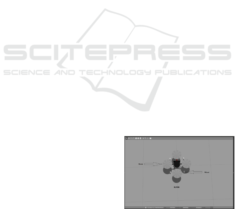
libraries and simulators. A simulation model of a
Figure 1: Visual model of HyFDR in Gazebo simulator.
ICINCO 2018 - 15th International Conference on Informatics in Control, Automation and Robotics
202
Quadcopter named as Hector Quadrotor was used.
This model is available as a ROS package. It runs
with Gazebo simulator in ROS environment.
Hector Quadrotor has a depth camera and a Laser
range finder attached to it. A hybrid vehicle named
as HyFDR was developed by addition of four
powered wheels to Hector Quadrotor model. The
simulation model of HyFDR in Gazebo is shown in
figure 1. The environmental constants and the
physical parameters of HyFDR are given in table 1.
Table 1: Parameters and constants for HyFDR.
Parameters Symbol Value
Mass of HyFDR m 1.477 Kg
Gravitational acceleration g
9.8m
Top area of HyFDR
0.5
Front area of HyFDR
0.022
Coefficient of rolling
friction
µ
0.06
Distance between nodes d 1m
Density of air ρ
1.22
Air drag coefficient
1.5
Tilt angle of HyFDR α 20 degrees
Radius of propeller r 0.127m
Velocity of HyFDR v
1m
A virtual world in Gazebo simulator was created
by using built-in models of houses, trees, and terrain.
Later some obstacles were placed in this virtual
world to create different scenarios for navigation.
The size, amount and position of obstacles are
important factors, which affect the locomotion mode
of HyFDR. The virtual world is shown in figure 2.
Figure 2: Custom world and obstacles in Gazebo.
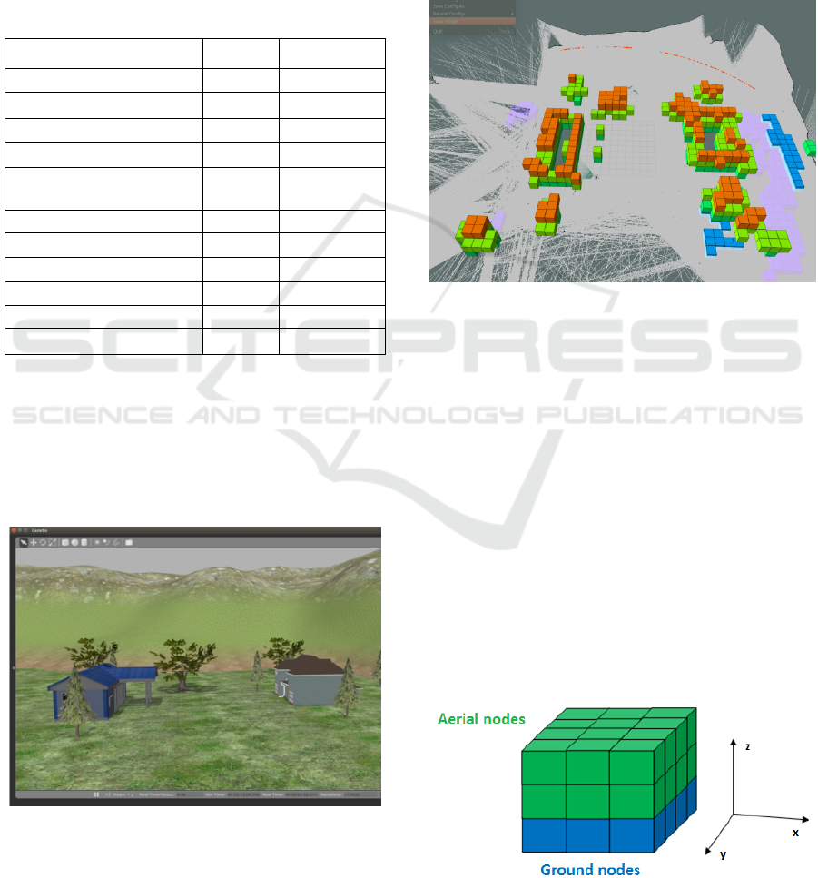
Gmapping and Octomap are the ROS packages
used to make 3D map of the virtual world. The map
was saved as a binary format. The final 3D map of
the virtual world is shown in figure 3. HyFDR is
placed at the centre of the map. The start position
and target position were marked. To find the path
from start position to destination, we used node
based path finding method, known as A* algorithm.
It finds the shortest path from start position to the
destination. The modified A* algorithm finds the
path with least energy consumption. To implement
the A* algorithm, the map has to be divided into a
gird of three dimensional nodes.
Figure 3: Map of the environment.
A* algorithm requires G-cost, H-cost and F-cost
of the adjacent nodes, to find the shortest path. The
G-cost of adjacent node is the sum of the G-cost for
current node and the movement cost for adjacent
node. The movement cost is the energy required to
move from current node to its adjacent node (Yang,
2016). Considering Manhattan distance, the distance
between current node and its adjacent node is one
meter. A 3D node grid is created as shown in figure
4. The x-axis and y-axis contains positive and
negative values. HyFDR is not allowed to go below
the ground, so the z-axis contains only positive
values. HyFDR has two modes of locomotion: flying
in air and driving on ground. This 3D node grid
contains two major types of nodes: Aerial nodes
(green colored cubes) and Ground nodes (blue
colored cubes).
Figure 4: A 3D node grid.
Energy Efficient Path Planning of Hybrid Fly-Drive Robot (HyFDR) using A* Algorithm
203
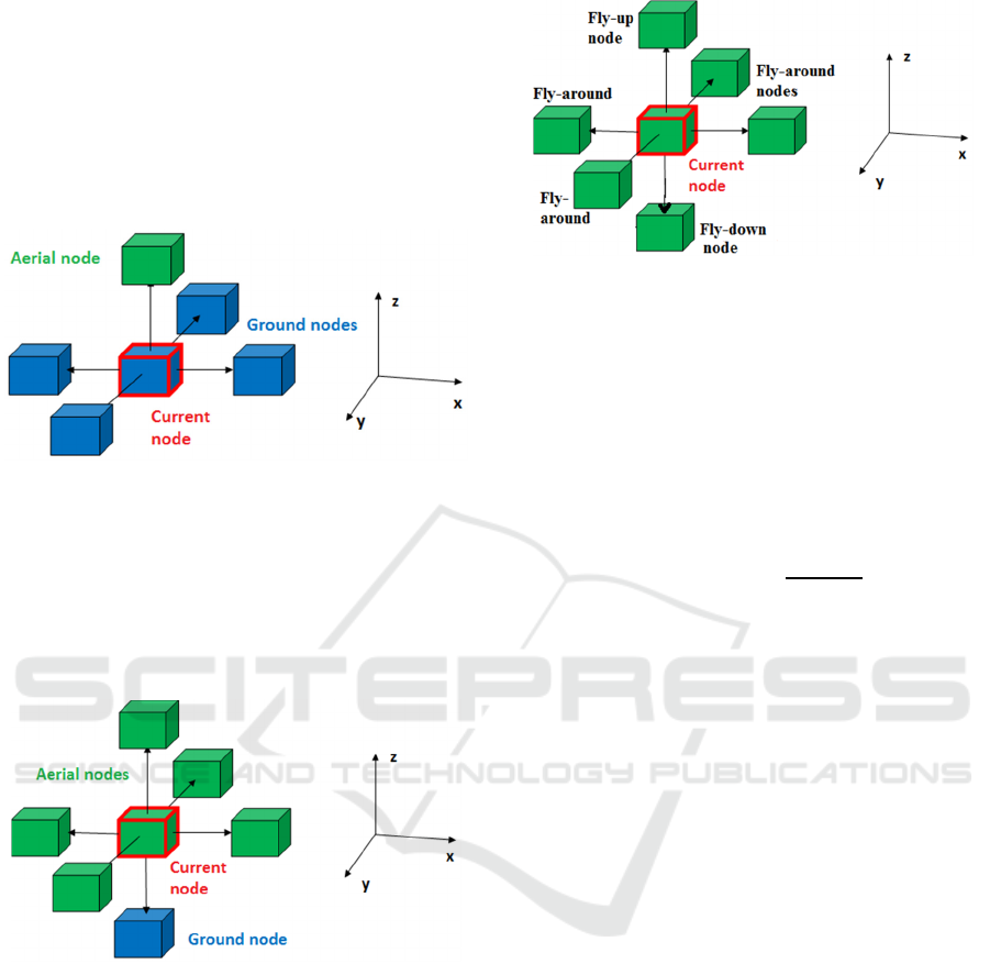
Considering Manhattan distance, during driving
mode, each current node (blue colored cube with red
edges) will have five neighboring nodes as shown in
figure 5. There are four nodes on the sides of the
current node, they are named as Ground nodes (blue
colored cubes). There is only one node on the top of
current node and it is called Aerial node (green
colored cube).
Figure 5: Neighboring nodes during ground locomotion.
During flight mode each current node will have six
neighboring nodes, as shown in figure 6. Four nodes
(green colored cubes) surrounding the current node
in xy-plane and one node on the top of current node
are Aerial nodes. The node below the current node is
a Ground node.
Figure 6: Neighboring nodes during aerial locomotion.
During the flight mode, HyFDR will be
travelling through Aerial nodes. Depending upon the
direction of motion, Aerial nodes are further divided
into three categories: Fly-up nodes, Fly-down nodes,
and Fly-around nodes as shown in figure 7. When
the HyFDR is flying vertically upward then the
Aerial nodes in the path will be named as Fly-up
nodes. When the HyFDR is flying in horizontal
direction along x-axis or y-axis, then the nodes in
the path will be named as Fly-around nodes. When
the HyFDR is flying down vertically, then the Aerial
nodes in the path will be named as Fly-down nodes.
Figure 7: Three types of Aerial nodes.
2.1 Movement Cost for Ground Nodes
The movement cost of Ground nodes (
) is the
amount of energy spend to travel a distance of one
meter while driving on ground. This energy is
consumed to overcome the rolling friction of wheels
on the ground and against the air drag. It can be
calculated by using following equation:
=μ+
(1)
where m is the mass of HyFDR, g is gravitational
acceleration, μ is the coefficient of rolling friction, d
is the distance between two adjacent nodes,
is the
air drag coefficient,
is the front area of HyFDR,
is the density of air and v is the velocity of HyFDR
on ground. On the right side of equation 1, all the
quantities are constants except velocity v. By
substituting the values of constants from table 1,
following equation is obtained:
= 0.87+0.02v
(2)
In real life scenario the velocity v of HyFDR will be
a variable quantity, which may change from node to
node, but we assumed that HyFDR will drive with
constant velocity of 1m
through all ground
nodes. Substituting the velocity in equation 2, gives
= 0.89 joules.
2.2 Movement Cost for Aerial Nodes
The Movement cost for aerial nodes can be
calculated by finding the energy consumption during
flight. During Quadcopter's flight, most of energy is
consumed in hovering and some of energy is
consumed against air drag. The energy required
against downward gravitational pull is called
hovering energy
. This energy provides a constant
upward pull and prevent the Quadcopter from falling
ICINCO 2018 - 15th International Conference on Informatics in Control, Automation and Robotics
204

down on ground. When the Quadcopter is in
hovering state the thrust produced by its propellers is
equal to the weight of Quadcopter (Leishman, 2006).
Hovering energy per node can be calculated using
the following equation:
=
(3)
where m is the mass of HyFDR, g is gravitational
acceleration, is the density of air, d is the distance
between two nodes, v is the velocity of HyFDR
during flight and r is the radius of propeller. The
right side of the equation 2 has all constants
quantities except velocity v. Substituting the values
of these constants from table 1 in equation 2, we get
hovering energy:
=
(4)
for v = 1m
, we get the hovering energy per node
equal to 77 joules.
2.2.1 Movement Cost for Fly-up Nodes
The energy required to fly vertically upward from
current node to its above node is the movement cost
for Fly-up nodes
. It is the sum of potential
energy, hovering energy and the energy required to
overcome air drag. It can be calculated using
following equation:
=
+
+
(5)
where
is the energy required to hover per node, m
is the mass of HyFDR, g is gravitational
acceleration, is the density of air, d is the distance
between two nodes, v is the velocity of HyFDR
during flight,
is the top area of HyFDR and
is
the air drag coefficient. By substituting the values of
constants from table 1, we get:
=14.5+
+0.46v
(6)
for v = 1m
, we get the
equal to 91.95 joules.
2.2.2 Movement Cost for Fly-down Nodes
The energy consumed by HyFDR to move vertically
downward from current node to its adjacent below
node is called movement cost for Fly-down node.
This energy is equal to hovering energy minus the
energy given by air drag. In this case the air drag
force and the hovering force are acting in upward
direction but the gravitational pull force and the
motion of HyFDR are in downward direction. To
calculate the movement cost for Fly-down nodes, we
used following equation:
=
−
(7)
where
is the energy required to hover per node, m
is the mass of HyFDR, g is gravitational
acceleration, is the density of air, d is the distance
between two nodes, v is the velocity of HyFDR
during vertical downward flight,
is the top area of
HyFDR and
is the air drag coefficient. By
substituting the values of constants from table 1, we
get:
=
−0.46v
(8)
for v = 1m
, we get the
almost equal to 76.54
joules.
2.2.3 Movement Cost for Fly-around Nodes
The energy consumed by HyFDR while flying
horizontally is called the movement cost for Fly-
around nodes and it is represented by the symbol
. During horizontal flight HyFDR consumes
most of energy for hovering in air and some energy
against the air drag force. The movement cost for
Fly-around nodes can be calculated using following
equation:
=
+
α
(9)
where
is the energy required to hover per node,
is the density of air, d is the distance between two
nodes, v is the velocity of HyFDR during horizontal
flight,
is the effective area of HyFDR, α is the tilt
angle of HyFDR and
is the air drag coefficient.
The tilt angle α and the velocity v are the variable
quantities but other terms are constants. After
substituting the values of the constants from table 1,
we get:
=
+0.45αv
(10)
for α=20degrees, v = 1m
, we get the
equal to 77.15 joules.
Energy Efficient Path Planning of Hybrid Fly-Drive Robot (HyFDR) using A* Algorithm
205

In real world scenarios, the movement cost will
not be a constant quantity. It will change with the
speed of HyFDR, its tilt angle, the type of terrain,
the slope of ground and the wind speed. In our case
we assumed that the velocity of the HyFDR will be
constant through the path, the ground surface is
smooth, homogeneous and without any slope. The
movement cost for all type of nodes are summarized
in the following table:
Table 2: Movement cost for different type of nodes.
Node type Symbol value
Ground node
0.89 J
Fly-up node
91.95 J
Fly-down node
76.54 J
Fly-around node
77.15 J
2.2.4 Arbitrary Movement Cost
The movement costs can be assigned arbitrarily to
specific nodes to get the desired path. If the map
contains smooth and rough terrain then we can
assign a high movement cost to rough terrain so that
HyFDR will avoid driving on rough terrain. If we
want to completely avoid driving on ground, then we
can assign movement cost to Ground nodes that is
larger than the movement cost for aerial nodes. In
this case the HyFDR will only fly to reach target
position. In general if the less energy consumption
during locomotion is desired then assign the Ground
nodes a small movement cost and a high movement
cost to Aerial nodes. If fast locomotion is desired
then assign a high movement cost to Ground nodes
and a low movement cost to Aerial nodes.
2.2.5 Movement Cost for Quadcopter
For comparison purpose, we have also calculated the
movement cost for Quadcopter. The Quadcopter
without wheels has a mass of 1.3 kg but the other
parameters will remain similar to HyFDR. We have
used similar method to calculate the movement cost
for Aerial nodes as we did for HyFDR. In case of
Quadcopter there will be no Ground nodes. The
movement cost for Fly-around nodes is 65.15 joules,
the movement cost for Fly-down node is 64.54 and
the movement cost for Fly-up nodes is 77.95 joules.
2.3 Calculation of G-cost
In A* algorithm, the G-cost is the distance of the
current node from the start node. It ensures the
search of shortest path (Tan, 2016). The G-cost for
the adjacent node is the sum of the G-cost of current
node and the movement cost of the adjacent node.
2.4 Calculation of H-cost
In A* algorithm, H-cost (heuristic cost) is the
distance between the current node and target node.
H-cost makes the search faster. The H-cost is
calculated by finding a Manhattan distance between
current node and the target node. We assumed that
the target is always located on the ground. The H-
cost of adjacent node will depend upon the current
node and the type of adjacent node. If the current
node is Ground node then we shall use following
equation to find the H-cost:
=
−
+
−
(11)
where
is the movement cost for Ground nodes,
,
are the coordinates of the current node and
,
are the coordinates for the target node.
If the current node is Aerial node and the
adjacent node is Fly-down node then we shall use
following equation to find the H-cost:
=
−
+
−
+
−
(12)
where
is the movement cost for Ground nodes,
,
,
are the coordinates of the current node and
,
,
are the coordinates for the target node.
is the movement cost for Fly-down node.
If the current node is Aerial node and the
adjacent node is Fly-around node, then to calculate
the H-cost we shall use following equation:
=
−
+
−
+
−
(13)
where
,
,
are the coordinates of the current
node and
,
,
are the coordinates for the target
node.
is the movement cost for Fly-down node
and
is the movement cost for Fly-around node.
2.5 Calculation of F-cost
After getting the G-cost and H-cost for each adjacent
node around the current node, the algorithm will
calculate F-cost by adding G-cost and H-costs. The
node which has minimum value of F-cost will be
selected. This process will be repeated until the
ICINCO 2018 - 15th International Conference on Informatics in Control, Automation and Robotics
206
target node is reached and the path with minimum
energy consumption is discovered.
This energy efficient path will be translated into
motion by motion algorithm. The motion list is
generated from start node to the target node. The
motions are driven by proportional (P) controllers,
which gets the position feedback from the ground
truth. If the desired position is achieved then the
algorithm moves to the next motion in the motion
list. This process will continue up to the last item in
the motion list, resulting in the navigation of HyFDR
to the target node on the map.
3 EXPERIMENT AND RESULTS
We created a virtual world in Gazebo as shown in
figure 9. The task is to deliver a mail from the post
office to the house with help of the HyFDR. The
start position for HyFDR is in front of post office
and the target position is in front of the house. The
shortest distance between the start position and the
target position is 9 meters. We created three test
cases by changing the position and amount of
obstacles in the path. The height, length and the
width of each building block of obstacle is one
meter.
3.1 Test Case 1
In the first test case, a boundary wall (obstacle) was
created by joining the blocks around the post office
as shown in figure 9. The red line shows the path
followed by HyFDR from start point to target during
autonomous navigation. It started by driving on the
ground, after travelling a distance of 4 meters, it
reached near boundary wall. It switched to flight
mode and flew vertically upward for one meter, then
flew horizontally for two meters. After passing the
boundary wall, it flew down on the ground and
switched to driving mode again. Finally it reached
target position after driving three meters. During the
navigation, HyFDR covered a distance of 11 meters.
It navigated through seven Ground nodes, one Fly-
up node, two Fly-around nodes and one Fly-down
node. The movement cost for all these nodes has
been already calculated. The total energy consumed
during navigation can be calculated by addition of
movement costs of the respective nodes present in
the path. HyFDR consumed 329.02 joules of energy
during the navigation in this map.
Figure 8: Simulation in Gazebo for test case 1.
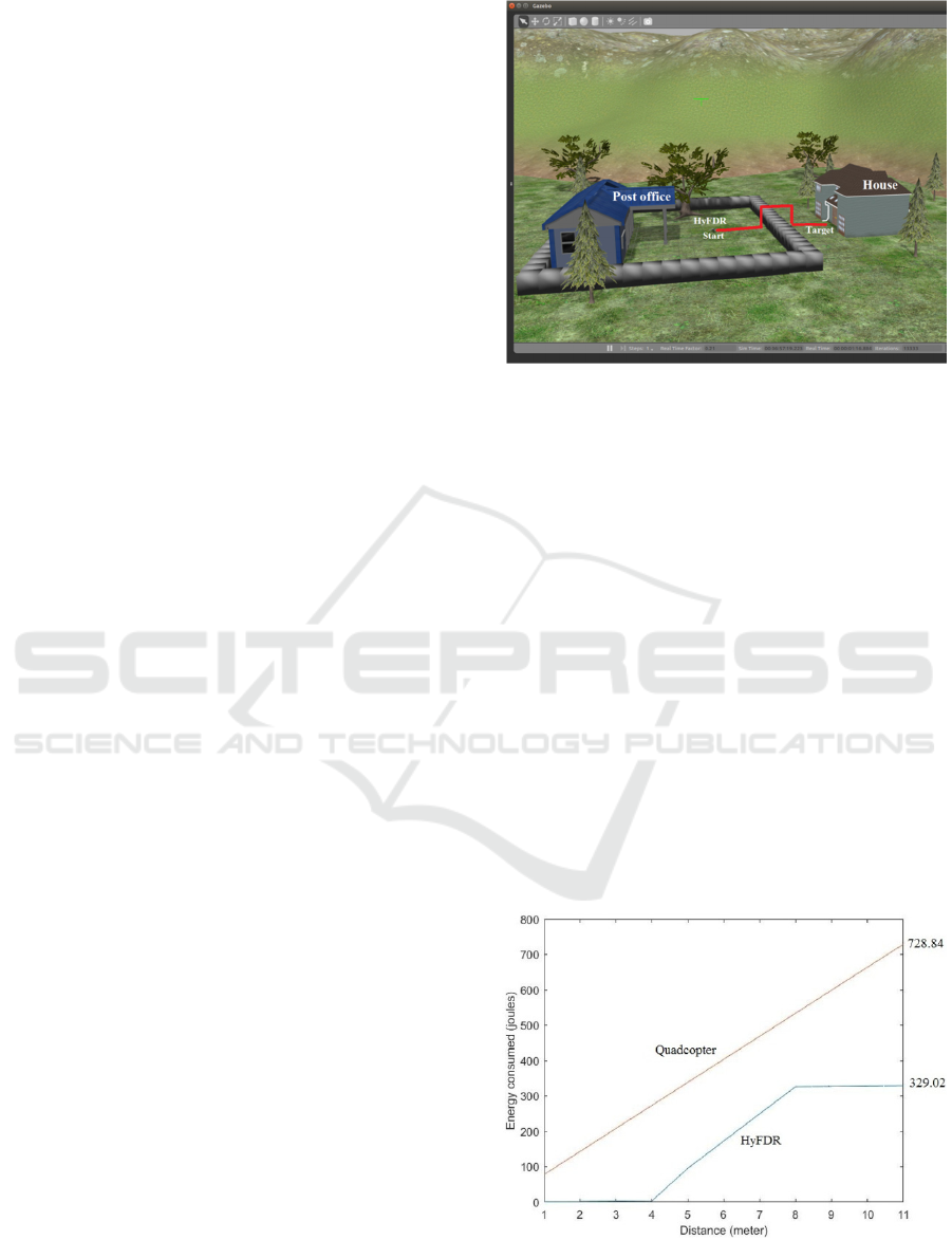
The movement costs for Aerial nodes of
Quadcopter are given in section 2.2.5. For the same
virtual world as shown in figure 9, we did path
planning for a theoretical Quadcopter. The virtual
world has same start position, obstacles, and target
position. The Quadcopter can only use Aerial nodes
during navigation. In this scenario, for takeoff it
used one Fly-up node, then it flew horizontally
through nine Fly-around nodes and finally it passes
through one Fly-down node for landing. It traveled a
total distance of 11 meters. The total energy
consumed by Quadcopter is the sum of the
movement costs of nodes used in the path. The
theoretical Quadcopter consumed 728.84 joules of
energy. A comparison of energy consumed by a
Quadcopter and HyFDR is shown in figure 9.
Despite of a small increase in weight due to wheels,
HyFDR consumed 399.82 joules less energy as
compared to Quadcopter.
Figure 9: Comparison of energy consumption.
Energy Efficient Path Planning of Hybrid Fly-Drive Robot (HyFDR) using A* Algorithm
207
In figure 9, it can be seen that during flight mode
the slope of the graph for HyFDR is slightly steeper
than the graph of Quadcopter. This shows that,
HyFDR consumed more energy during flight as
compared to quadcopter. The increased energy
consumption during flight is caused by additional
weight of wheels. This test case shows that the
energy consumption during flight can be reduced by
switching to driving mode on ground, whenever
there is a opportunity for driving is available. Flying
consumes 87 times more energy as compared to
driving on ground. During autonomous navigation if
the movement cost of Ground nodes is less, then the
A* algorithm makes the HyFDR to drive on ground
more frequently. This reduces the total energy
consumption during autonomous navigation.
3.2 Test Case 2
In the second test case a wall (obstacle) was placed
between the start point and the target as shown in the
figure 10. In this test environment, HyFDR has
multiple options (paths) to reach the target. It can
navigate by flight, driving or combination of both.
The modified A* algorithm always find the path
with lowest energy consumption, and in this case,
the path for driving on ground is available and it
requires least energy consumption. During
simulation HyFDR used only single mode of
locomotion (driving) and followed the driving path
(red line) as shown in figure 10. It travelled a total
distance 25 meters. It consumed 22.25 joules of
energy during navigation on ground. The energy
consumption during navigation can be calculated by
multiplying the total distance covered with the
movement cost of Ground node.
Figure 10: Gazebo world simulation for test case 2.
The results of this simulation showed that if there
is a driving path on ground available, then HyFDR
will only drive on ground. The reason for this
behavior is the low movement cost of Ground nodes
and high movement cost of Aerial nodes. The path
followed by HyFDR in test case 2 requires minimum
energy consumption but it is not the shortest path.
The shortest path was in test case 1, where HyFDR
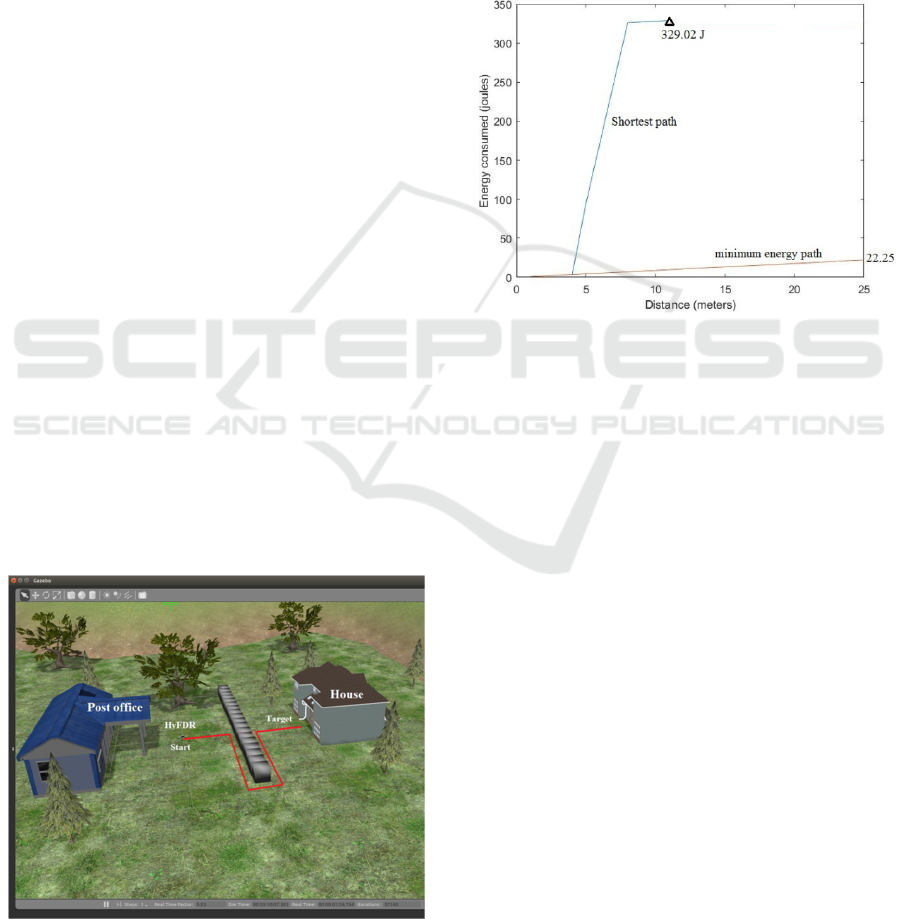
used dual mode of locomotion. Figure 11 shows the
comparison of path followed by HyFDR in test case
1 and the path followed by HyFDR in test case 2.
Figure 11: Comparison of energy consumption.
Figure 11 shows that with dual mode
locomotion, HyFDR navigated through the shortest
path, travelled a distance of 11 meters and consumed
329.02 joules of energy. But with driving mode it
travelled a distance of 25 meters and consumed
22.25 joules of energy. It implies that in case of dual
mode of locomotion the shortest path is not always
energy efficient path. The drive only path saves
energy but it is longer path and requires more time
to reach the target point. The flight only path
provides fast locomotion but it is energy expansive.
A combination of flight and driving gives optimum
results with respect to energy saving and time
saving.
3.3 Test Case 3
This test case is not related to energy efficiency,
instead it is designed to show the use of arbitrary
movement cost for Ground and Aerial nodes. It has
been mentioned in section 2.2.4, that the movement
cost can be arbitrarily assigned to nodes based on
their type and location. The virtual world shown in
figure 12, has a rough terrain between post office
and house. To avoid the driving on rough terrain, it
is desired that HyFDR should only fly during
ICINCO 2018 - 15th International Conference on Informatics in Control, Automation and Robotics
208
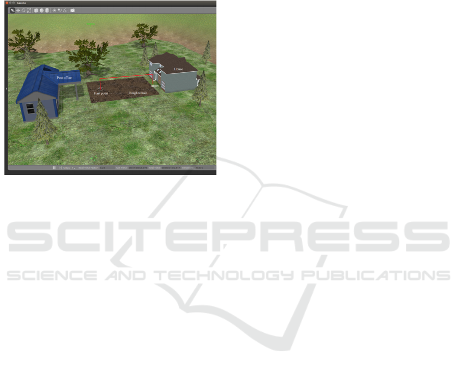
autonomous navigation. To achieve this purpose, the
movement cost of Ground nodes were made much
higher than the movement cost of Aerial nodes. The
path followed by HyFDR is shown as red line in
figure 12. It only used flight mode during navigation
from start point to target.
Figure 12: Gazebo world simulation for test case 3.
It is obvious from these experiments that
movement cost of nodes decides whether the
HyFDR will fly air or drive on ground during
autonomous navigation. If the movement cost of
Ground nodes is smaller than movement cost of
Aerial nodes then the HyFDR will be energy
efficient but will take more time to reach target. If
the movement cost of Aerial nodes is less than
Ground nodes then HyFDR will be less energy
efficient but requires less time to reach the target. To
get the optimum results with respect to energy
efficiency and travelling time, the movement cost of
Ground nodes and Aerial nodes can be arbitrarily
assigned depending upon the position, size and
number of obstacles in the path.
4 CONCLUSION
The energy consumption by a Quadcopter during
locomotion can be reduced by giving it the ability to
drive on ground. Addition of wheels to a Quadcopter
increases its weight, and causes a slight increases in
energy consumption during flight, but due to its
ability to drive on ground, its overall energy
efficiency increases. Our modified A* algorithm
finds energy efficient path and influences the
locomotion mode of HyFDR, forcing it to frequently
drive on ground during autonomous navigation.
Depending upon the obstacles and terrain, the
movement costs of nodes can be arbitrarily assigned
to achieve optimum results with respect to travel
time and energy consumption.
REFERENCES
Bautista, L., M., Tinbergen, J., & Kacelnik, A. 2001. To
walk or to fly? How birds choose among foraging
modes. In Proceedings of the National Academy of
Sciences of the United States of America, 98(3), 1089–
1094.
Dietrich, T., Krug, S., and Zimmermann, A. 2017. An
empirical study on generic multicopter energy
consumption profiles. In 2017 Annual IEEE
International Systems Conference (SysCon), Montreal,
QC, pp. 1-6.
Jones, K., Boria, F., Bachmann, R., Vaidyanathan, R., Ifju,
P., and Quinn, R. 2006. MMALV - The Morphing
Micro Air-Land Vehicle. In 2006 IEEE/RSJ
International Conference on Intelligent Robots and
Systems, Beijing, China, pp. 5-5.
Daler, Ludovic & Mintchev, Stefano & Stefanini, Cesare
& Floreano, Dario. 2015. A bioinspired multi-modal
flying and walking robot. In Bioinspiration &
biomimetics. Bioinspiration &biomimetics. 10.
016005. 10.1088/1748-3190/10/1/016005.
Mulgaonkar, Y., et., al. 2016. The flying monkey: A
mesoscale robot that can run, fly, and grasp. In 2016
IEEE International Conference on Robotics and
Automation (ICRA), Stockholm,, pp. 4672-4679.
Kalantari, A., and Spenko, M., 2014. Modelling and
Performance Assessment of the HyTAQ, a Hybrid
Terrestrial/Aerial Quadrotor. In IEEE Transactions on
Robotics, vol. 30, no. 5, pp. 1278-1285.
Page, R., J., and Pounds, I., E., P., 2014. The Quadroller:
Modelling of a UAV/UGV hybrid quadrotor. In
IEEE/RSJ International Conference on Intelligent
Robots and Systems, Chicago, IL, 2014, pp. 4834-
4841.
Araki, B., Strang, J., Pohorecky, S., Qiu, C., Naegeli, T.,
& Rus, D. 2017. Multi-robot path planning for a
swarm of robots that can both fly and drive. In 2017
IEEE International Conference on Robotics and
Automation (ICRA), 5575-5582.
Hart, P., E., Nilsson, N., J., Raphael, B. 1968. A Formal
Basis for the Heuristic Determination of Minimum
Cost Paths. In IEEE Transactions on Systems Science
and Cybernetics SSC4. 4 (2): 100–107.
Yang, L., Qi, J., Song, D., Xiao, J., Han, J., and Xia, Y.
2016. Survey of Robot 3D Path Planning Algorithms.
In J. Control Sci. Eng. 2016 (March 2016), 5.
Tan, J., Zhao, L., Wang, Y., Zhang, Y., and Li, L. 2016.
The 3D Path Planning Based on A* Algorithm and
Artificial Potential Field for the Rotary-Wing Flying
Robot. In 8th International Conference on Intelligent
Human-Machine Systems and Cybernetics (IHMSC),
Hangzhou, pp. 551-556.
Energy Efficient Path Planning of Hybrid Fly-Drive Robot (HyFDR) using A* Algorithm
209

Romli, I., F., and Yaakob, S., M. 2014. Personal air
vehicle (PAVE) application in Malaysia. In
International Conference on Advanced Logistics and
Transport (ICALT), Hammamet, pp. 59-64.
Rajashekara, K., Wang, Q., and Matsuse, Q. 2016. Flying
Cars: Challenges and Propulsion Strategies. In IEEE
Electrification Magazine, vol. 4, no. 1, pp. 46-57.
Leishman, J., G. 2006. Principles of Helicopter
Aerodynamics, Cambridge University Press. New
York, 2nd edition.
ICINCO 2018 - 15th International Conference on Informatics in Control, Automation and Robotics
210
