Autonomous Vehicle Steering Wheel Estimation from a Video using

Multichannel Convolutional Neural Networks

Arthur Emidio T. Ferreira

, Ana Paula G. S. de Almeida

and Flavio de Barros Vidal

Department of Computer Science, University of Brasilia, Brazil

Department of Mechanical Engineering, University of Brasilia, Brazil

Keywords:

Multichannel Convolutional Neural Networks, Vehicle Steering Wheel Estimation, Autonomous Vehicles.

Abstract:

The navigation technology in autonomous vehicles is an artiﬁcial intelligence application which remains un-

solved and has been signiﬁcantly explored by the automotive and technological industries. Many image pro-

cessing and computer vision techniques allow signiﬁcant improvements on such recent technologies. Using

this motivation as a basis, this work proposes a novel methodology based on Multichannel Convolutional

Neural Networks (M-CNN) capable of estimating the steering angle of an autonomous vehicle, having as only

input images captured by a camera attached to the vehicle’s frontal area. We propose ﬁve Convolutional Neural

Network architectures: 1-channel, 2-channel and 3-channel in the convolution step. Based on the performed

tests using a public video dataset, it is presented a quantitative comparison between the proposed models.

1 INTRODUCTION

Nowadays, autonomous driving and navigation

technology in autonomous vehicles is an artiﬁcial in-

telligence application that has drawn great attention

with the popularity of intelligent vehicles. In these

application areas, unsolved issues still remain and

have been signiﬁcantly explored by the automotive

and technological industries, due to the potential im-

pact that such innovation will bring in the near future

(Pomerleau, 1989; Thrun et al., 2006; Thorpe et al.,

1988).

Over the last decades, many works have approa-

ched this theme: In 1989, (Pomerleau, 1989) descri-

bed the construction of an autonomous vehicle based

on artiﬁcial neural networks. The proposed network is

responsible for providing guidance to the vehicle and

the architecture of the network consists of a classical

artiﬁcial neural network (ANN) with a single interme-

diate layer, containing 29 neurons fully connected to

the input units.

Many works involving ANN in autonomous vehi-

cle applications can be found in the vast litera-

ture available. However, a lot has changed since

the advent of new network architectures. With the

rise of deep learning, Convolutional Neural Net-

works (CNN) have improved the image comprehen-

sion tasks by learning more discriminative features,

allowing an useful development on several systems,

including autonomous vehicles (Wang et al., 2018).

We will describe a small sample of the numerous

applications of these networks architectures as fol-

lows: in (Chen et al., 2015) it is proposed an autono-

mous navigation system called DeepDriving based on

CNN. The speed, acceleration, brake and steering an-

gle are computed from the CNN output values, which

are then used as input to an algorithm that describes

the control logic of the vehicle.

The works of (Bojarski et al., 2016) and (Bojarski

et al., 2017) propose a CNN called PilotNet capable

of estimating the steering angle of a vehicle. In or-

der to observe the features extracted by PilotNet, a

deconvolution-based algorithm (Zeiler et al., 2011) is

used. It ﬁnds regions of the image that have the hig-

hest levels of activation in the maps produced by the

convolution layers of the network. The PilotNet net-

work was tested in a car and was able to carry out a

15 minute journey in urban area without human inter-

vention by 98% of the time.

Finally, in this work we propose a novel approach

to construct new models based on Multichannel Con-

volutional Neural Networks (M-CNN) that are capa-

ble of estimating the steering angle of a vehicle given

only a set of images from its frontal view, which is

a task that many autonomous vehicle systems must

solve.

To reach this main objective, the sections of this

work are divided as follows: Section 2 describes in

Ferreira, A., Almeida, A. and Vidal, F.

Autonomous Vehicle Steering Wheel Estimation from a Video using Multichannel Convolutional Neural Networks.

DOI: 10.5220/0006920605170524

In Proceedings of the 15th International Conference on Informatics in Control, Automation and Robotics (ICINCO 2018) - Volume 2, pages 517-524

ISBN: 978-989-758-321-6

517

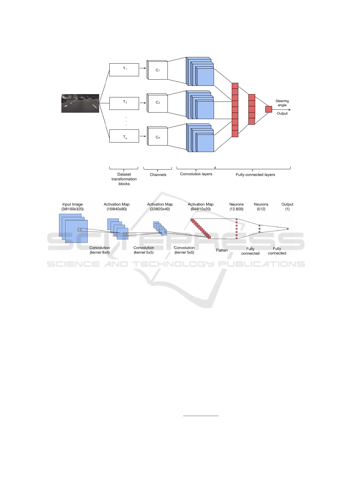
(a) Proposed M-CNN architecture.

(b) Base CNN architecture diagram.

Figure 1: Details of the proposed M-CNN architecture.

details the proposed methodology. In Section 3 the

results are shown and discussed. Section 4 is dedica-

ted to conclusions and further works.

2 PROPOSED METHODOLOGY

As seen in the related works presented in Section 1,

artiﬁcial neural networks have presented promising

results in the construction of many parts of autono-

mous vehicles systems. Hence, in this work we pro-

pose a novel method based on multichannel convolu-

tional neural networks capable of estimating a vehi-

cle’s steering angle using only information from real

trafﬁc video scenes. In this speciﬁc case, the develo-

ped system receives as input a collection of RGB ima-

ges captured using a dash cam placed inside the vehi-

cle and outputs the estimated steering angle at the gi-

ven instant, meeting the requirements of autonomous

vehicles.

2.1 Dataset

Based on the proposed methodology, illustrated on Fi-

gure 1-(a), a dataset provided by the comma.ai organi-

zation

is used. The dataset is composed of 11 videos

with a 320x160 pixels resolution, variable duration

and captured in a 20Hz frequency using a dash cam

installed inside the vehicle (i.e. Acura ILX 2016),

capturing frames of its frontal vision while driving

during day and night periods, usually on a highway.

In total, the dataset is composed of 522,434 frames,

resulting in approximately 7 hours of recording time.

For the purposes of this work, the only information

that was taken into account was the video frames (in

RGB format) and the steering angle values. The steer-

ing angle is given in degrees and corresponds to the

rotation angle of the vehicle’s steering wheel. Every

angle value present in the dataset belongs to the inter-

val [−502.3, 512.6].

The dataset is made available on the CC BY-NC-SA

3.0 license.

ICINCO 2018 - 15th International Conference on Informatics in Control, Automation and Robotics

518

2.2 CNN Architecture

According to (Goodfellow et al., 2016), CNNs are

specialized artiﬁcial neural networks that process in-

put data with some kind of spatial topology, such as

images, videos, audio and text. Also in (Goodfellow

et al., 2016), an artiﬁcial neural network is conside-

red convolutional when it has at least one convolution

layer and receives a multidimensional input (also re-

ferred as a tensor) and applies a series of convolutions

using a set of ﬁlters. In addition to convolution layers,

CNNs are usually composed of other types of layers.

2.2.1 Multichannel CNNs

Multichannel CNNs (M-CNNs) are commonly adop-

ted when some sort of parallel processing of the input

data is desired. Such streams can eventually merge

into one in the latter layers of the network.

In recent works (Baccouche et al., 2011; Ji et al.,

2013), it is common for the point of concatenation to

be present before the ﬁrst fully connected layer of the

network, that is, the parallel processing is concentra-

ted between the convolution layers. Action recogni-

tion, for example, is a problem that has been explored

with M-CNNs due to the difﬁculty of traditional CNN

in handling temporal information from input videos.

It is proposed in (Karpathy et al., 2014) a multi-

channel methodology capable of generating labels of

the main action in a video. In (Karpathy et al., 2014),

a 2-channel CNN is proposed, each channel receiving

two frames of the input video. Another advantage of

using M-CNNs is also highlighted by (Karpathy et al.,

2014) and it consists in reducing the dimensionality

of the network input, which helps to decrease the pro-

cessing time.

2.2.2 Architecture

The objective of the proposed approach is to basically

solve a regression problem: estimate the steering an-

gle given a set of images. Therefore, this work uses

as base a preexisting single channel CNN architecture

proposed by the comma.ai organization, described by:

Figure 1-(b) presents the diagram of the base

CNN. In more details, the network contains 13 lay-

ers and has 6,621,809 parameters to be learned. In

topological order, the layers are described by:

1. Normalization: an image in the RGB format is

given as input to the CNN, such that the value of

every pixel belongs to the interval [0, 255]. The

ﬁrst layer of the network is responsible for nor-

malizing the pixel values to range [−1, 1]. Thus,

the following operation is executed:

127.5

− 1 (1)

Output dimension: 3 × 160 × 320

2. Convolution Layer (CONV): the parameters of

the ﬁrst convolution layer are present in Table 1.

Table 1: Parameters of the ﬁrst convolution layer.

of kernels Kernel dimension Stride 0-padding

16 8 × 8 4 × 4 2

Output dimension: 16 × 40 × 80

3. ELU

Output dimension: 16 × 40 × 80

4. Convolution Layer (CONV): the parameters of

the second convolution layer are present in Table

Table 2: Parameters of the second convolution layer.

of kernels Kernel dimension Stride 0-padding

32 5 × 5 2 × 2 2

Output dimension: 32 × 20 × 40

5. ELU

Output dimension: 32 × 20 × 40

6. Convolution Layer (CONV): the parameters of

the third convolution layer are present in Table 3.

Table 3: Parameters of the third convolution layer.

of kernels Kernel dimension Stride 0-padding

64 5 × 5 2 × 2 2

Output dimension: 64 × 10 × 20

7. Flatten: ﬂattens the input data. For example, if

the input has a 100x42 dimension, the output will

be a R

4200

vector. This step is done so that the spa-

tial information learned through the convolution

steps can be transferred to fully-connected layers.

Output dimension: 1 × 12, 800

8. Dropout: the dropout layer was originally propo-

sed by Srivastava et al. (Srivastava et al., 2014),

and it is used as a form of regularization to pre-

vent the occurrence of overﬁtting. This layer is

used just in the training phase, and its operation

consists in setting a value of 0 for each unity with

a probability of p.

Dropout probability: 20%

Output dimension: 1 × 12, 800

Autonomous Vehicle Steering Wheel Estimation from a Video using Multichannel Convolutional Neural Networks

519

9. ELU

Output dimension: 1 × 12, 800

10. Fully-connected layer (FC)

Output dimension: 1 × 512

11. Dropout: as in the previous dropout layer, it is

used only in the training step.

Dropout probability: 50%

Output dimension: 1 × 512

12. ELU

Output dimension: 1 × 512

13. Fully-connected Layer (FC): the last layer of the

CNN is fully connected with the 512 units from

the previous layer. It outputs h ∈ R, which con-

sists in the vehicle’s steering angle at the moment

the input image was captured.

Output dimension: 1 × 1

2.3 Proposed Architectures

From the base architecture presented in Subsection

2.2.2, this work proposes the construction of two

CNNs composed of multiple input channels, as shown

in Figure 1-(a). The motivation behind the idea is to

observe the impact that M-CNNs have in solving the

supervised problem of estimating a vehicle’s steering

angle, incorporating temporal and spatial information

obtained by the camera.

Following the original CNN architecture descri-

bed in Figure 1-(b), we propose a multichannel model

that processes the inputs in different channels until the

last ELU layer. In other words, the outputs of the last

ELU layers from each channel are concatenated and

are passed as input to the ﬁrst fully connected layer.

2.4 Developed Models

After deﬁning the dataset and the CNN architectures,

we now propose a framework used to generate all mo-

dels trained from scratch that are able to receive a set

of input images captured in a given instant by a vehi-

cle’s dash cam and output an estimation of the steer-

ing angle in such moment.

The proposed framework primarily consists in

modifying the original dataset to allow the multichan-

nel networks to be trained. Afterwards, 5 distinct ty-

pes of models are trained. Lastly, the trained models

can be tested and evaluated. More details about these

models are described in Section 2.4.2.

2.4.1 Dataset Preparation

The base CNN proposed by comma.ai has a single in-

put channel. Given that the methodology of this work

proposes the usage of M-CNNs (C1 for channel 1, C2

for channel 2 and C3 for channel 3), the original da-

taset (for future references, we will denote the origi-

nal dataset as BASE 1) had to be adapted, generating

four more versions of datasets. All these generated

datasets were inspired in the work developed by (Kar-

pathy et al., 2014) and are described as follows:

• BASE 2: original frame (C1) + frame subsampled

in 50% (C2).

• BASE 3: original frame (C1) + central region of

the image in original scale (C2).

• BASE 4: original frame (C1) + frame subsampled

in 50% (C2) + central region of the image in ori-

ginal scale (C3).

• BASE 5: frame subsampled in 50% (C1) + central

region of the image in original scale (C2).

Notice that the central region takes a 50% portion

of the original frame.

2.4.2 Training Models

Five different models were trained, each one used one

of the dataset versions presented in Section 2.4.1 and

are described as follows:

Model 1 (trained with BASE 1): In this model, the

original single channel CNN is used. This is done

for comparison with the other proposed models as a

reference model.

Model 2 (trained with BASE 2): The second model

uses the two-channel CNN architecture. In one chan-

nel it receives the original image and in the other one

it receives the same frame subsampled in 50%. He-

reby, we can observe how the CNN behaves with the

input given in different scales.

Model 3 (trained with BASE 3): The third model

uses the two-channel CNN architecture. In the ﬁrst

channel it receives the original image and in the se-

cond channel it receives the original image’s central

ROI. Based on this model, we can observe how the

neural network can react when receiving a region of

the frame that probably contains objects closer to the

vehicle and that are present in the same road lane.

Model 4 (trained with BASE 4): The fourth model

uses the three-channel CNN architecture. The ob-

jective behind this model is to observe whether the

neural network can produce better results if the ad-

ditional information provided in models 2 and 3 are

ICINCO 2018 - 15th International Conference on Informatics in Control, Automation and Robotics

520

given as input at the same time, combined with the

original frame.

Model 5 (trained with BASE 5): The ﬁfth model

uses the two-channel CNN architecture and it was ba-

sed on the idea of multi-resolution CNNs proposed by

Karpathy et al. (Karpathy et al., 2014), which introdu-

ces two input channels: fovea and context. The fovea

channel receives the central ROI of the input frame

in original resolution (resulting in a 160x80 ROI in

our dataset). The context channel receives the image

subsampled in 50% (also containing a 160x80 reso-

lution in our dataset). Thereby, the dimensionality of

the CNN input is halved, which can present a better

performance in terms of training time. Therefore, the

ﬁfth model is proposed to observe the impact on how

M-CNNs can cause when receiving input with infor-

mation loss.

3 EXPERIMENTAL RESULTS

This section presents the results obtained based on the

datasets and CNN architectures detailed in the met-

hodology. The GPU used for training the proposed

models was an NVIDIA GeForce GTX 1070 and all

models were developed using the TensorFlow (Abadi

et al., 2015) and Keras (Chollet et al., 2015) frame-

works.

The performed experiments correspond to the

tests of the ﬁve models presented in the previous

section. Each model was trained in 200, 350 and 500

epochs, such that the epoch size is 10,000 examples.

Each training session with N epochs was repeated 3

times and each time the dataset was randomly partiti-

oned in training/validation/test subsets, following the

70/15/15 proportion schema.

Given that the proposed CNNs output the steering

angle using raw image data as input, it is crucial that

the model’s accuracy is correctly evaluated. All va-

lues presented in this section correspond to the error

that each trained model had for their corresponding

test set. The error is calculated between the estima-

ted vehicle’s steering angle and the ground truth angle

obtained with an internal sensor, which is provided by

the database.

The error measurement generally used to evaluate

the prediction of numerical values is the root of the

mean squared error (RMSE), which is described by:

RMSE =

∑

i=1

− y

)

(2)

where n corresponds to the number of predictions, y

equals to the ground truth angle of the i-th example

and y

is the predicted steering angle given by the

CNN’s output. Thus, the lower the RMSE is, the gre-

ater is the model’s generalization capacity. In order

to enable the comparison between models trained un-

der different combinations of subsets, the normalized

form of the RMSE (NRMSE) was chosen. It is evalu-

ated in Equation 3:

NRMSE =

RMSE

max

− y

min

(3)

where y

min

and y

max

correspond to the lowest and gre-

atest angle values observed in the test set, respecti-

vely.

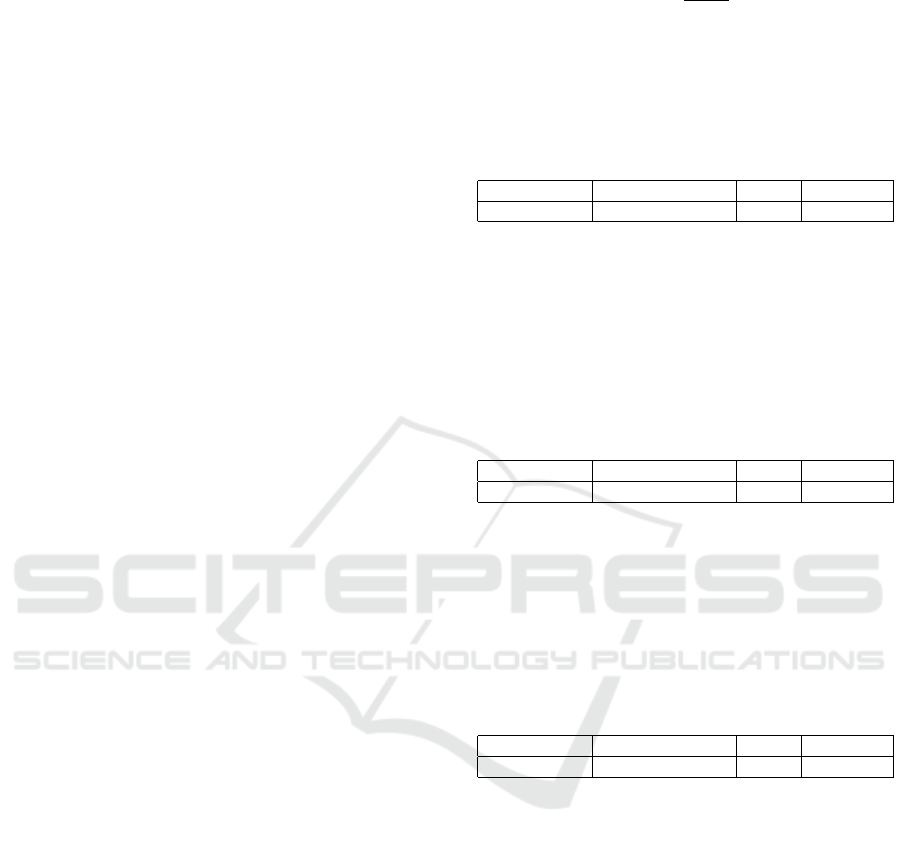
The values described in Table 4 shows the average

of the obtained NRMSE errors and the lowest values

for each epoch are highlighted. The graph presented

in Figure 2 shows the average of the obtained NRMSE

errors.

Table 4: Average test errors of all trained models.

200 350 500

Model 1 0.057548 0.047214 0.048096

Model 2 0.040906 0.046397 0.047917

Model 3 0.048535 0.038011 0.047673

Model 4 0.047513 0.046985 0.051179

Model 5 0.048974 0.051207 0.052770

3.1 Discussion

Based on the results obtained for each model present

in Figure 2, it is observed that the NRMSE values for

the multichannel models are similar between each ot-

her. However, it can be observed that the proposed

models have better performance when compared to

the reference model (i.e. Model 1). It is possible to

notice that the Model 3 trained for 350 epochs presen-

ted an average NRMSE of 0.038010, 7.07% less than

the second best model (i.e. Model 2 trained for 200

epochs).

Figures 3-(a) up to (e) show how the estimated an-

gles compare to the ground truth on some test videos.

It can be seen that the predicted angles are likely to

match the direction from the ground truth. Additio-

nally, it is observed that the models output subtle va-

riations in the steering wheel. Through the test charts,

it is also noted that the error is more expressive at the

beginning and end of the tests. This is due to the fact

that in the used database, the ends of the videos corre-

spond to the moment of entry and exit of the vehicle

inside a garage, an event that implies a great variation

in the steering angle.

On average, the models trained for 500 epochs did

not bring improvements in the results. Thus, it is ex-

Autonomous Vehicle Steering Wheel Estimation from a Video using Multichannel Convolutional Neural Networks

521

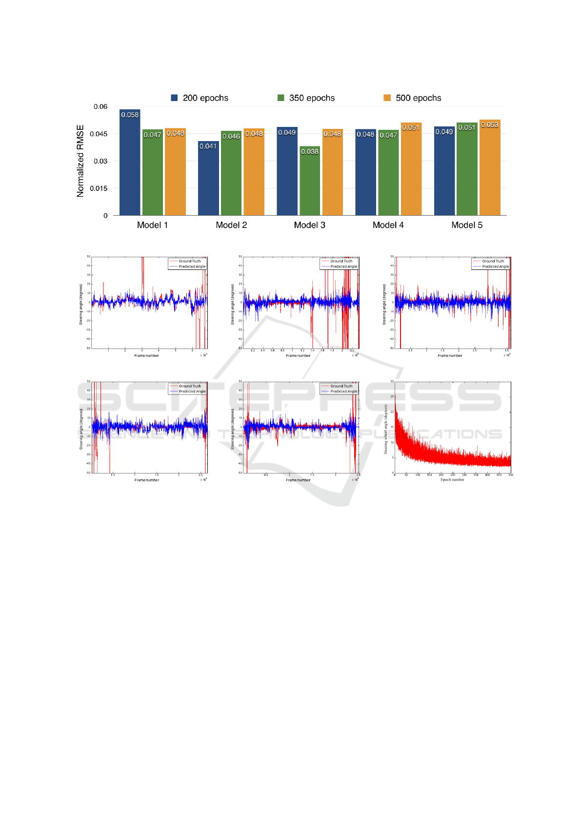
Figure 2: Average test errors of all trained models.

(a) (b) (c)

(d) (e) (f)

Figure 3: Figures (a) up to (e) show predicted outputs for models 1 up to 5 respectively trained for 200 epochs. In (f) it is

shown the training error variation of Model 5 trained for 500 epochs.

pected that the model should suffer from overﬁtting

when trained with more epochs, losing its capacity

for generalization. For example, notice in Figure 3-

(f) the training error of Model 5 trained for 500 epo-

chs. It can be seen that the error does not signiﬁcantly

decrease after 200 epochs.

Finally, it is possible to perform a qualitative eva-

luation of the proposed models, following the idea

described in (Karpathy et al., 2014), by visualizing

the activation maps given as output by one of the con-

volution layers. Hence, Figure 4-(b) shows 16 acti-

vation maps produced by the ﬁrst convolution layer

from Model 1 trained for 200 epochs, given the frame

on Figure 4-(a) as input to the network.

With the activation maps in Figure 4-(b), it is ob-

served that the ﬁlters from the ﬁrst convolution layer

highlight the lane marks. In other words, the CNN

was able to detect the presence of visual elements in

the scene without being previously programmed to

perform such task. By ﬁnding the lane marks (Figure

4-(b)), it is possible that the network was able to learn

that the vehicle should keep itself between them while

estimating the steering angles.

4 CONCLUSIONS AND FURTHER

WORKS

This work proposes a methodology based on M-CNN

that is able to estimate the steering angle of a vehicle

ICINCO 2018 - 15th International Conference on Informatics in Control, Automation and Robotics

522

(a) Frame corresponding to the activation maps.

(b) Activation maps produced by the ﬁrst convolution layer.

Figure 4: Activation maps from Model 1 trained for 200 epochs.

using only videos as input. As seen in Section 3, it

is possible to observe that the third proposed model

trained with 350 epochs obtained a lower NRMSE

when compared to the others, including the single

channel as reference model. Speciﬁcally in this mo-

del, it can be seen that M-CNNs provide signiﬁcant

improvements in their use in autonomous vehicle ap-

plications. The performance of the best model was

approximately 7% better than the reference model.

Furthermore, the ﬁfth model presents results simi-

lar to the others, showing that it was capable of main-

taining robustness even when receiving an input with

reduced dimensionality.

Future works may include the addition of explicit

space-time information during the training stage, cre-

ating new versions of datasets and training models,

exploring how M-CNNs architecture respond to this

information. Also, new datasets and more complex

situations must be tested to validate the approach.

REFERENCES

Abadi, M., Agarwal, A., Barham, P., Brevdo, E., Chen, Z.,

Citro, C., Corrado, G. S., Davis, A., Dean, J., De-

vin, M., Ghemawat, S., Goodfellow, I., Harp, A., Ir-

ving, G., Isard, M., Jia, Y., Jozefowicz, R., Kaiser,

L., Kudlur, M., Levenberg, J., Man

e, D., Monga, R.,

Moore, S., Murray, D., Olah, C., Schuster, M., Shlens,

J., Steiner, B., Sutskever, I., Talwar, K., Tucker, P.,

Vanhoucke, V., Vasudevan, V., Vi

egas, F., Vinyals, O.,

Warden, P., Wattenberg, M., Wicke, M., Yu, Y., and

Zheng, X. (2015). TensorFlow: Large-scale machine

learning on heterogeneous systems. Software availa-

ble from tensorﬂow.org.

Baccouche, M., Mamalet, F., Wolf, C., Garcia, C., and Bas-

kurt, A. (2011). Sequential deep learning for human

action recognition. In International Workshop on Hu-

man Behavior Understanding, pages 29–39. Springer.

Bojarski, M., Testa, D. D., Dworakowski, D., Firner, B.,

Flepp, B., Goyal, P., Jackel, L. D., Monfort, M., Mul-

ler, U., Zhang, J., Zhang, X., Zhao, J., and Zieba,

K. (2016). End to end learning for self-driving cars.

CoRR, abs/1604.07316.

Bojarski, M., Yeres, P., Choromanska, A., Choroman-

ski, K., Firner, B., Jackel, L. D., and Muller, U.

(2017). Explaining how a deep neural network trai-

ned with end-to-end learning steers a car. CoRR,

abs/1704.07911.

Chen, C., Seff, A., Kornhauser, A. L., and Xiao, J. (2015).

Deepdriving: Learning affordance for direct percep-

tion in autonomous driving. CoRR, abs/1505.00256.

Autonomous Vehicle Steering Wheel Estimation from a Video using Multichannel Convolutional Neural Networks

523

Chollet, F. et al. (2015). Keras. https://github.com/fchollet/

keras.

Goodfellow, I., Bengio, Y., and Courville, A. (2016). Deep

Learning. MIT Press.

Ji, S., Xu, W., Yang, M., and Yu, K. (2013). 3d convolu-

tional neural networks for human action recognition.

IEEE transactions on pattern analysis and machine

intelligence, 35(1):221–231.

Karpathy, A., Toderici, G., Shetty, S., Leung, T., Sukthan-

kar, R., and Fei-Fei, L. (2014). Large-scale video

classiﬁcation with convolutional neural networks. In

CVPR.

Pomerleau, D. A. (1989). Alvinn: An autonomous land

vehicle in a neural network. In Touretzky, D. S., editor,

Advances in Neural Information Processing Systems

1, pages 305–313. Morgan-Kaufmann.

Srivastava, N., Hinton, G., Krizhevsky, A., Sutskever, I.,

and Salakhutdinov, R. (2014). Dropout: A simple way

to prevent neural networks from overﬁtting. J. Mach.

Learn. Res., 15(1):1929–1958.

Thorpe, C., Hebert, M., Kanade, T., and Shafer, S. (1988).

Vision and navigation for the carnegie-mellon navlab.

10(3):362 – 373.

Thrun, S., Montemerlo, M., Dahlkamp, H., Stavens, D.,

Aron, A., Diebel, J., Fong, P., Gale, J., Halpenny,

M., Hoffmann, G., Lau, K., Oakley, C., Palatucci, M.,

Pratt, V., Stang, P., Strohband, S., Dupont, C., Jen-

drossek, L.-E., Koelen, C., Markey, C., Rummel, C.,

van Niekerk, J., Jensen, E., Alessandrini, P., Bradski,

G., Davies, B., Ettinger, S., Kaehler, A., Neﬁan, A.,

and Mahoney, P. (2006). Stanley: The robot that won

the darpa grand challenge. Journal of Field Robotics,

23(9):661–692.

Wang, Q., Gao, J., and Yuan, Y. (2018). Embedding struc-

tured contour and location prior in siamesed fully

convolutional networks for road detection. IEEE

Transactions on Intelligent Transportation Systems,

19(1):230–241.

Zeiler, M. D., Taylor, G. W., and Fergus, R. (2011). Adap-

tive deconvolutional networks for mid and high level

feature learning. In 2011 International Conference on

Computer Vision, pages 2018–2025.

ICINCO 2018 - 15th International Conference on Informatics in Control, Automation and Robotics

524