Iterated Algorithmic Bias in the Interactive Machine Learning Process of
Information Filtering
Wenlong Sun
1
, Olfa Nasraoui
1
and Patrick Shafto
2
1
Dept of Computer Engineering and Computer Science, University of Louisville, Louisville, KY, U.S.A.
2
Dept of Mathematics and Computer Science, Rutgers University - Newark, Newark, NJ, U.S.A.
Keywords:
Information Retrieval, Machine Learning, Bias, Iterative Learning.
Abstract:
Early supervised machine learning (ML) algorithms have used reliable labels from experts to build predicti-
ons. But recently, these algorithms have been increasingly receiving data from the general population in the
form of labels, annotations, etc. The result is that algorithms are subject to bias that is born from ingesting
unchecked information, such as biased samples and biased labels. Furthermore, people and algorithms are
increasingly engaged in interactive processes wherein neither the human nor the algorithms receive unbiased
data. Algorithms can also make biased predictions, known as algorithmic bias. We investigate three forms of
iterated algorithmic bias and how they affect the performance of machine learning algorithms. Using control-
led experiments on synthetic data, we found that the three different iterated bias modes do affect the models
learned by ML algorithms. We also found that Iterated filter bias, which is prominent in personalized user
interfaces, can limit humans’ ability to discover relevant data.
1 INTRODUCTION
Websites and online services offer large amounts of
information, products, and choices. This information
is only useful to the extent that people can find what
they are interested in. There are two major adaptive
paradigms aiming to help sift through information:
information retrieval (Robertson, 1977; Spark, 1978)
and recommender systems(Pazzani and Billsus, 1997;
Cover and Hart, 1967; Koren et al., 2009; Abdollahi
and Nasraoui, 2014; Goldberg et al., 1992; Nasraoui
and Pavuluri, 2004; Abdollahi and Nasraoui, 2016;
Abdollahi, 2017; Abdollahi and Nasraoui, 2017). All
existing approaches aid people by suppressing infor-
mation that is determined to be disliked or not rele-
vant. Thus, all of these methods, by gating access to
information, have potentially profound implications
for what information people can and cannot find, and
thus what they see, purchase, and learn.
Common to both recommender systems and in-
formation filters is: (1) selection of a subset of data
about which people express their preference by a pro-
cess that is not random sampling, and (2) an itera-
tive learning process in which people’s responses to
the selected subset are used to train the algorithm for
subsequent iterations. The data used to train and op-
timize performance of these systems are based on hu-
man actions. Thus, data that are observed and omitted
are not randomly selected, but are the consequences
of people’s choices.
1.1 Iterated Learning and Language
Evolution
In language learning, humans form their own map-
ping rules after listening to others, and then speak the
language following the rules they learned, which will
affect the next learner (Kirby et al., 2014). Language
learning and machine learning have several properties
in common. For example, a ‘hypothesis‘ in language
is analogous to a ‘model‘ in machine learning. Le-
arning a language which gets transmitted throughout
consecutive generations of humans is analogous to le-
arning an online model throughout consecutive itera-
tions of machine learning.
Researchers have shown that iterated learning can
produce meaningful structure patterns in language le-
arning (Kirby et al., 2014; Smith, 2009). In particu-
lar, the process of language evolution can be viewed
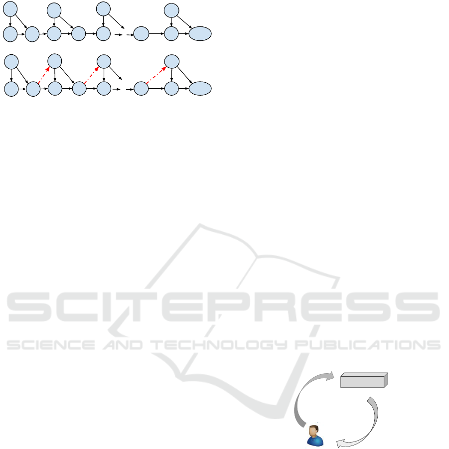
in terms of a Markov chain, as shown in Figure 1 (a).
We should expected an iterated learning chain to con-
verge to the prior distribution of all hypotheses given
that the learner is a Bayesian learner (Griffiths and
110
Sun, W., Nasraoui, O. and Shafto, P.
Iterated Algorithmic Bias in the Interactive Machine Learning Process of Information Filtering.
DOI: 10.5220/0006938301100118
In Proceedings of the 10th International Joint Conference on Knowledge Discovery, Knowledge Engineering and Knowledge Management (IC3K 2018) - Volume 1: KDIR, pages 110-118
ISBN: 978-989-758-330-8
Copyright © 2018 by SCITEPRESS – Science and Technology Publications, Lda. All rights reserved

x
0
h
1
y
0
y
1
x
2
x
1
y
2
h
2
y
n
x
n
h
n+1
h
n
...
(a) A Markov Chain
x
0
h
1
y
0
y
1
x
2
x
1
y
2
h
2
y
n
x
n
h
n+1
h
n
...
(b) Not defined and referred in the text
Figure 1: Illustration of iterated learning with (bottom) and
without (top) dependency from previous iterations.
Kalish, 2005). That is, the knowledge learned is not
accumulated during the whole process. We refer to
this iterated learning model as pure iterated learning
(PIL).
1.2 Relationship between Iterated
Algorithmic Bias and other Types of
Bias
In statistics, bias refers to the systematic distortion of
a statistic. Here we can distinguish a biased sam-
ple, which means a sample that is incorrectly assu-
med to be a random sample of a population, and es-
timator bias, which results from an estimator whose
expectation differs from the true value of the parame-
ter (Rothman et al., 2008). Within our scope, bias
is closer to the sample bias and estimator bias from
statistics; however, we are interested in what we call
iterated algorithmic bias which is the dynamic bias
that occurs during the selection by machine learning
algorithms of data to show to the user to request la-
bels in order to construct more training data, and
subsequently update their prediction model, and how
this bias affects the learned (or estimated) model in
successive iterations.
Recent researches pointed to the need to pay atten-
tion to bias and fairness in machine learning (McNair,
2018; Goel et al., 2018; Friedler et al., 2018; Klein-
berg et al., 2018; Dwork et al., 2018). Some rese-
arch has studied different forms of biases, some are
due to the algorithms while others are due to inherent
biases in the input data or in the interaction between
data and algorithms (Hajian et al., 2016; Baeza-Yates,
2016; Baeza-Yates, 2018; Lambrecht and Tucker,
2018; Garcia, 2016; Bozdag, 2013; Spinelli and Cro-
vella, 2017; Chaney et al., 2017; Jannach et al., 2016).
Some work studied biases emerging due to item popu-
larity (Joachims et al., 2017; Collins et al., 2018; Li-
ang et al., 2016; Schnabel et al., 2016). A recent work
studied bias that is due to the assimilation bias in re-
commender systems (Zhang et al., 2017). Because
recommender systems have a direct impact on hu-
mans, some recent research studied the impact of po-
larization on biasing rating data (Badami et al., 2017)
and proposed strategies to mitigate this polarization
in collaborative filtering recommender systems (Ba-
dami et al., 2018) while other recent research pointed
to bias emerging from continuous feedback loops be-
tween recommender systems and humans (Shafto and
Nasraoui, 2016; Nasraoui and Shafto, 2016). Over-
all, the study of algorithmic bias falls under the um-
brella of fair machine learning (Abdollahi and Nasra-
oui, 2018).
Taking all the above in consideration, we observe
that most previous research has treated algorithmic
bias as a static factor, which fails to capture the ite-
rative nature of bias that is born from continuous in-
teraction between humans and algorithms. We argue
that algorithmic bias evolves with human interaction
in an iterative manner, which may have a long-term
effect on algorithm performance and humans’ disco-
very and learning. We propose a framework for in-
vestigating the implications of interactions between
humans and algorithms, that draws on diverse litera-
ture to provide algorithmic, mathematical, computa-
tional, and behavioral tools for investigating human-
algorithm interaction. Our approach draws on foun-
dational algorithms for selecting and filtering of data
from computer science, while also adapting mathe-
matical methods from the study of cultural evolu-
tion (Griffiths and Kalish, 2005; Beppu and Griffiths,
2009) to formalize the implications of iterative inte-
ractions.
Algorithm
Biased output
Biased Input
Figure 2: Evolution of bias between algorithm and human.
A continuous interaction between humans and algorithms
generates bias that we refer to as iterated bias, namely bias
that results from repeated interaction between humans
and algorithms.
In this study, we focus on simulating how the data
that is selected to be presented to users affects the al-
gorithm’s performance (see Figure 2). In this work,
we choose recommendation systems as the machine
learning algorithm to be studied. One reason is that
recommendation systems have more direct interaction
options with humans, while information retrieval fo-
cuses on getting relevant information only. We further
simplify the recommendation problem into a 2-class
classification problem, namely, like/relevant (class 1)
Iterated Algorithmic Bias in the Interactive Machine Learning Process of Information Filtering
111

or dislike/non-relevant (class 0), thus focusing on a
personalized content-based filtering recommendation
algorithm.
2 ITERATED ALGORITHMIC
BIAS IN ONLINE LEARNING
Because we are interested in studying the interaction
between machine learning algorithms and humans,
we adopt an efficient way to observe the effect from
both sides by using iterated interaction between algo-
rithm and human action.
To begin, we consider three possible mecha-
nisms for selecting information to present to users:
Random, Active-bias, and Filter-bias. These three
mechanisms simulate different regimes. Random se-
lection is unbiased and will be used here purely as a
baseline for no filtering. Active-bias selection intro-
duces a bias whose goal is to accurately predict user’s
preferences. Filter-bias selection brings a bias whose
goal is to provide relevant information or preferred
items.
Before we go into the three forms of iterated algo-
rithmic bias, we first investigate PIL. We adopt some
of the concepts from Griffiths (Griffiths and Kalish,
2005). Consider a task in which the algorithm le-
arns a mapping from a set of m inputs X = {x
1
,...,x
m
}
to m corresponding outputs {y
1
,...,y
m
} through a la-
tent hypothesis h. For instance, based on previous
purchase or rating data (x,y), a recommendation sy-
stem will collect a new data about a purchased item
(x
new,
y
new
) and update its model to recommend more
interesting items to the users. Here, x represents the
algorithm’s selections and y represents people’s re-
sponses (e.g. likes/dislikes). Following Griffiths’ mo-
del for human learners, we assume a Bayesian model
for prediction.
2.1 Iterated Learning with Iterated
Filter-bias Dependency
The extent of the departure that we propose from a
conventional machine learning framework toward a
human - machine learning framework, can be measu-
red by the contrast between the evolution of iterated
learning without and with the added dependency (see
Figure 1).
We used notation q(x) to represent this indepen-
dence. Here, q(x) indicates an unbiased sample from
the world, rather than a selection made by the algo-
rithm. On the other hand, with the dependency, the al-
gorithm at iteration n sees input x
n
which is generated
from both the objective distribution q(x) and another
distribution p
seen
(x|h
n
) that captures the dependency
on the previous hypothesis h
n
which implies future
bias of what can be seen by the user. Thus, the proba-
bility of input item x is given by:
p(x|h
n
) = (1 − ε)p
seen
(x|h
n
) + εq(x) (1)
Here ε is the weight of two factors which control the
data that algorithm will see. Recall that the probabi-
lity of seeing an item is related to its rank in a rating
based recommendation system or an optimal proba-
bilistic information filter (Robertson, 1977). In most
circumstances, the recommendation system has a pre-
ferred goal, such as recommending relevant items
(with y=1). Then x will be chosen based on the proba-
bility of relevance p(y = 1|x,h
n
), x ∈ X. Assume that
we have a candidate pool X at time n (In practice X
would be the data points or items that the system can
recommend at time n), then
p
seen
(x|h
n
) =
p(y = 1|x, h
n
)
∑
x∈X
p(y = 1|x, h
n
)
(2)
The selection of inputs depends on the hypothesis,
and therefore information is not unbiased, p(x|h
n
) 6=
q(x). The derivations of the transition probabilities in
Eq. 2 will be modified to take into account Eq. 1, and
will become
p(h
n+1
|h
n
) =
∑
x∈X
∑
y∈Y
p(h
n+1
|x,y)p(y|x,h
n
)p
seen
(x|h
n
)
(3)
Eq. 3 can be used to derive the asymptotic behavior
of the Markov chain with transition matrix T (h
n+1
) =
p(h
n+1
|h
n
), i.e.
p(h
n+1
) = εp(h
n+1
) + (1 − ε)T
bias
(4)
Here, T
bias
is:
"
∑
x∈X
∑
y∈Y
p(h
n+1
|x,y)
∑
h
n
∈H
p(y|x,h
n
)p
seen
(x|h
n
)
#
p(h
n
)
(5)
Thus, iterated learning with filter bias converges to
a mixture of the prior and the bias induced by filtering.
To illustrate the effects of filter bias, we can analyze
a simple and most extreme case where the filtering
algorithm shows only the most relevant data in the
next iteration (e.g. top-1 recommender). Hence
x
top
= argmax
x
P(y|x,h) (6)
p
seen
(x|h
n
) =

1 f or x = x
top
0 otherwise

(7)
T
bias
=
"
∑
x∈X
∑
y∈Y
p(h
n+1
|x,y)
∑
h
n
∈H
p(y|x
top
n
,h
n
)
#
p(h
n
)
(8)
KDIR 2018 - 10th International Conference on Knowledge Discovery and Information Retrieval
112

Based on equation 3, the transition matrix is re-
lated to the probability of item x being seen by the
user, which is the probability of belonging to class
y = 1. The fact that x
top
n
maximizes p(y|x,h) sugge-
sts limitations to the ability to learn from such data.
Specifically, the selection of relevant data allows the
possibility of learning that an input that is predicted
to be relevant is not, but does not allow the possibility
of learning that an input that is predicted to be irre-
levant is actually relevant. In this sense, selection of
evidence based on relevance is related to the con-
firmation bias in cognitive science, where learners
have been observed to (arguably maladaptively) se-
lect data which they believe to be true (i.e. they fail
to attempt to falsify their hypotheses) (Klayman and
Ha, 1987). Put differently, recommendation algo-
rithms may induce a blind spot where data that are
potentially important for understanding relevance
are never seen.
2.2 Iterated Learning with Iterated
Active-bias Dependency
Active learning was first introduced to reduce the
number of labeled samples needed for learning an
accurate predictive model, and thus accelerate the
speed of learning towards an expected goal (Cohn
et al., 1996). Instead of choosing random samples to
be manually labeled for the training set, the algorithm
can interactively query the user to obtain the desired
data sample to be labeled (Settles, 2010).
p
active
(x|h) ∝ 1 − p(
ˆ
y|x,h) (9)
where
ˆ
y = argmax
y
(p(y|x,h)). Given x and h,
ˆ
y aims
to select the most certain predicted label, whether it is
class y=0 or class y=1. Hence in Eq. 9, x values are
selected to be the least certain about
ˆ
y, the predicted
y value.
Assuming a simplified algorithm where only the
very uncertain data are selected, we can investigate
the limiting behavior of an algorithm with the active
learning bias. Assuming a mixture of random sam-
pling and active learning, we obtain:
x
act
= argmax
x
(1 − p(
ˆ
y|x,h)) (10)
p(h
n+1
) = εp(h
n+1
) + (1 − ε)T
active
(11)
Where
T
active
=
"
∑
x∈X
∑
y∈Y
p(h
n+1
|x,y)
∑
h
n
∈H
p(y|x
act
n
,h
n
)
#
p(h
n
)
(12)
The limiting behavior depends on the iterated
active learning bias, x
act
n
. This is, in most cases, in
opposition to the goal of filtering, the algorithm will
only select data point(s) which are closest to the lear-
ned model’s boundary, if we are learning a classifier
for example. In contrast, the filtering algorithm is al-
most certain to pick items that it knows are relevant.
2.3 Iterated Learning with Random
Selection
The iterated random selection is considered as a tri-
vial baseline for comparison purposes. This selection
mechanism randomly chooses instances to pass to the
next learner during iterations.
2.4 Evaluating the Effect of Iterated
Algorithmic Bias on Learning
Algorithms
In order to study the impact of iterated bias on an al-
gorithm, we compute three properties: the blind spot,
boundary shift, and the Gini coefficient. These pro-
perties are defined below.
2.4.1 Blind Spot
The blind spot is defined as the set of data available
to a relevance filter algorithm for which, the probabi-
lity of being seen by the human interacting with the
algorithm that learned the hypothesis h, is less than δ:
D
F
δ
= {x ∈ X | p
seen
(x|h) < δ} (13)
In the real world, some data can be invisible to
some users because of bias either from users or from
the algorithm itself. Studying blind spots can enhance
our understanding about the impact of algorithmic
bias on humans. In addition, we define the class-1-
blind spot or relevant-item-blind spot as the data in
the blind spot, with true label y = 1
D
F+
δ
= {x ∈ D
F
δ
and y = 1)} (14)
Note that the blind spot in Eq. 13 is also called all-
classes-blind spot.
2.4.2 Boundary Shift
Boundary shift indicates how different forms of itera-
ted algorithmic bias affect the model h that is learned
by an algorithm. It is defined as the number of points
that are predicted to be in class y = 1 given a learned
model h:
b =
∑
x∈X
p(y = 1|x,h) (15)
Here b is the number of points that are predicted as
class y = 1 given a learned model h. This number
helps to quantify the extent of shift in the boundary as
a result of different bias modes.
Iterated Algorithmic Bias in the Interactive Machine Learning Process of Information Filtering
113

2.4.3 Gini Coefficient
We also conduct a Gini coefficient analysis on how
boundary shifts affect the inequality of predicted re-
levance for the test set. Let p
i
= p(y = 1|x
i
,h). For
a population with n values p
i
, i = 1 to n, that are in-
dexed in non-decreasing order ( p
(i)
≤ p
(i+1)
). The
Gini coefficient can be calculated as follows (Stuart
et al., 1994):
G = (
∑
n
i=1
(2i − n − 1)p
(i)
n
∑
n
i=1
p
(i)
) (16)
The higher the Gini coefficient, the more unequal are
the frequencies of the different labels. The Gini coef-
ficient is used to gauge the impact of different itera-
ted algorithmic bias modes on the heterogeneity of
the predicted probability in the relevant class during
human-machine learning algorithm interaction.
3 EXPERIMENTS
As stated in section 3, we mainly focus on a two-
class model of recommendation in order to perform
our study. In this situation, any classical supervised
classification could be used in our model (Domingos
and Pazzani, 1997; Hosmer Jr et al., 2013; Cortes and
Vapnik, 1995). For the purpose of easier interpreta-
tion and visualization of the boundary and to more
easily integrate with the probabilistic framework in
section 2, we chose the Naive Bayes classifier.
Synthetic Data: A 2D data set (see figure 3) was
generated from two Gaussian distributions correspon-
ding to classes y ∈ {0, 1} for like (relevant) and dislike
(non-relevant), respectively. Each class contains 1000
data points centered at {−2, 0} and {2, 0}, with stan-
dard deviation σ = 1. The data set is then split into
the following parts: Testing set: used as a global tes-
ting set (200 points from each class); Validation set:
used for the blind spot analysis (200 points from each
class). Note that the subset is similar to the testing set,
however we only use this one for blind spot analysis
to avoid confusion; Initializing set: used to initialize
the first boundary (we tested initialization with class
1/class 0 ratios as follows: 100/100). Note that ini-
tialization set can also be called initial training set;
Candidate set: used as query set of data which will
be gradually added to the training set (points besides
the above three groups that will be added to the can-
didate set).
The reason why we need the four subsets is that
we are simulating a real scenario with interaction
between humans and algorithms. Part of this inte-
raction will include picking query data items and la-
beling them, thus augmenting the training set. Thus,
Figure 3: Original data with two classes.
to avoid depleting the testing set, we need to isolate
these query items in the separate “candidate pool”. A
similar reason motivates the remaining separate sub-
sets in order to keep their size constant throughout all
the interactions of module learning.
Methods: We wish to simulate the human-algorithm
interaction at the heart of recommendation and in-
formation filtering. To do so, we initialize the mo-
dels following the initialization set. Then, we explore
three forms of iterated algorithmic bias modes (see
Section 2). We simulate runs of 200 iterations where
a single iteration is comprised of the algorithm provi-
ding a recommendation, the user labeling the recom-
mendation, and the algorithm updating its model of
the user’s preferences. Each combination of parame-
ters yields a data set that simulates the outcome of
human and algorithm interacting. We simulate this
whole process 40 times independently, which gene-
rates the data that we will use to investigate several
research questions.
4 RESULTS
The key issue is to study whether and how informa-
tion filtering may lead to systematic biases in the lear-
ned model, as captured by the classification boundary.
Based on the three metrics introduced in section 2.4,
we ask the question: How does iterated algorithmic
bias affect the learned categories?
To answer this question, we adopt four different
investigating approaches. First, we will compare the
inferred boundaries after interaction to the ground
truth boundaries. Second, we will focus on the effects
of iteration alone by analyzing the boundary before
interaction and after. Third, We use the Gini coeffi-
cient to measure the heterogeneity or inequality of the
predicted label distribution in the testing set. Fourth,
we investigate the size of the blind spot induced by
each of the iterated algorithmic bias modes. Together,
these will describe the outcomes of algorithmic bias,
in terms of the induced blind spot.
RQ 1: Do Different Forms of Iterated Algo-
KDIR 2018 - 10th International Conference on Knowledge Discovery and Information Retrieval
114

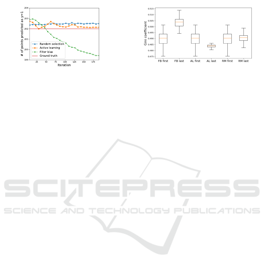
Figure 4: Boundary shift (Eq. 15) based on the three ite-
rated algorithmic bias forms. The y axis is the number of
testing points which are predicted to be in class y=1. The
iterated filter bias diverges from the ground truth signifi-
cantly with more iterations.
rithmic Bias Have Different Effects on the Boun-
dary Shift? To answer this question, We assume that
the initialization is balanced between both classes. As
shown in Eq. 1, we here assume that q(x) is identical
for all data points, thus we can ignore the second part
of the equation, i.e. the probability of being seen is
only dependent on the predicted probability of candi-
date points. Note that we could get some prior proba-
bility of X
i
, in which case we could add this parame-
ter to our framework. Here, we assume them to be the
same, hence we set ε = 0.
We wish to quantify differences in the boundary
between the categories as a function of the different
algorithm biases. To do so, we generate predictions
for each test point in the test set by labeling each point
based on the category that assigns it highest probabi-
lity. We investigate the proportion of test points with
the relevant label y = 1 at two time points: prior to
human-algorithm interactions (immediately after ini-
tialization), and after human algorithm interactions.
Note that we use ‘FB’ to represent filter bias, ‘AL’ for
active learning bias, and ’RM’ for random selection.
We run experiments with each of the three forms
of algorithm bias, and compare their effect on boun-
dary shifts. We also report the effect size based on
Cohen d (Cohen, 1988). In this experiment, the ef-
fect size (ES) is calculated by ES = (Boundary
t=0
−
Boundary
t=200
)/std(·), here std(·) is the standard de-
viation of the combined samples. We will use the
same strategy to calculate the effect size in the rest
of this paper. The results indicate significant differen-
ces for the filter bias condition (p < .001 by Mann-
Whitney test or t-test, effect size = 1.96). In contrast,
neither the Active Learning, nor the Random con-
ditions resulted in statistically significant differences
(p = .15 and .77 by Mann-Whitney test, or p = .84
and 1.0 by t-test; effective sizes .03 and 0.0, respecti-
vely).
To illustrate this effect, we plot the number of
points assigned to the target category versus ground-
Figure 5: Box-plot of the Gini coefficient resulting from
three forms of iterated algorithmic bias. The x-axis is the
iterated algorithmic bias modes. ‘First’ means the first ite-
ration (t=0), while ‘last’ indicates the last iteration (t=200).
An ANOVA test across these three iterated algorithmic bias
forms shows that the Gini index values are significantly dif-
ferent. The p-value from the ANOVA test is close to 0.000
(<0.05), which indicates that the three iterated algorithmic
bias forms have different effects on the Gini coefficient.
truth for each iteration. Figure 4 shows that random
selection and active learning bias converge to the
ground-truth boundary. Filter bias, on the other hand,
results in decreasing numbers of points predicted in
the target category class 1, consistent with an overly
restrictive category boundary.
RQ 2: Do Different Iterated Algorithmic Bias Mo-
des Lead to Different Trends in the Inequality of
Predicted Relevance throughout the Iterative Le-
arning Given the Same Initialization? To answer
this question, we run experiments with different forms
of iterated algorithmic bias, and record the Gini coef-
ficient when a new model is learned and applied to the
testing set during the iterations.
Although the absolute difference between the first
iteration and the last iteration is small (see Figure 5),
a one-way ANOVA test across these three iterated al-
gorithmic bias forms shows that the Gini index va-
lues are significantly different. The p-value from the
ANOVA test is close to 0.000 (< 0.05), which indica-
tes that the three iterated algorithmic bias forms have
different effects on the Gini coefficient.
Interpretation of this Result: Given that the Gini
coefficient measures the inequality or heterogeneity
of the distribution of the relevance probabilities, this
simulated experiment shows the different impact of
different iterated algorithmic bias forms on the hete-
rogeneity of the predicted probability to be in the rele-
vant class within human machine learning algorithm
interaction. Despite the small effect, the iterated algo-
rithmic bias forms affect this distribution in different
ways, and iterated filter bias causes the largest hete-
rogeneity level as can be seen in Figure 5. The fact
that filtering increases the inequality of predicted re-
levance means that filtering algorithms may increase
the gap between liked and unliked items, with a pos-
Iterated Algorithmic Bias in the Interactive Machine Learning Process of Information Filtering
115

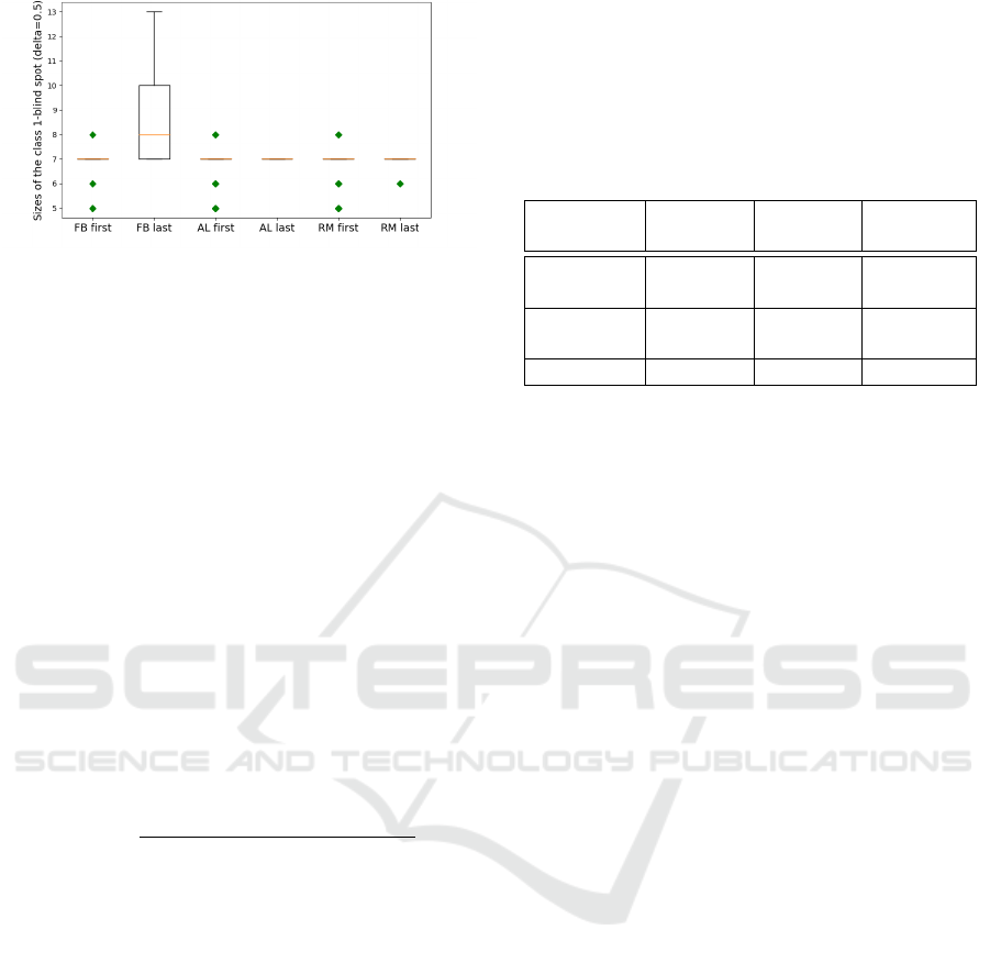
Figure 6: Box-plot of the size of the class-1-blind spot for
all three iterated algorithmic bias forms. In this figure, the
x-axis is the index of the three forms of iterated algorithms
biases, ‘First’ means the first iteration (t=0), while ‘last’ in-
dicates the last iteration (t=200). As shown in this box-plot,
the initial class-1-blind spot is centered at 7. This is because
the 200 randomly selected initial points from both classes
force the boundary to be similar regardless of the randomi-
zation.
sible impact on polarizing user preferences.
RQ 3: Does Iterated Algorithmic Bias Affect
the Size of the Class-1-blind Spot, i.e. is the Initial
Size of the Blind Spot D
F
δ
Significantly Different
Compared to Its Size in the Final Iteration? The
blind spot represents the set of items that are much
less likely to be shown to the user. Therefore this rese-
arch question studies the significant impact of an ex-
treme filtering on the number of items that can be seen
or discovered by the user, within human - algorithm
interaction. If the size of the blind spot is higher, then
iterated algorithmic bias results in hiding items from
the user. In the case of the blind spot from class 1,
this means that even relevant items are affected.
We run experiments with δ = 0.5, and record the
size of the class-1-blind spots with three different ite-
rated algorithmic bias forms. Here, we aim to check
the effect of each iterated algorithmic bias form. As
shown in Table 1, filter bias has significant effects
on the class-1-blind spot, while random selection and
active learning do not have a significant effect on the
class-1-blind spot size (see Figure 6). The negative
effect from iterated filter bias implies a large incre-
ase in the class 1 blind spot size, effectively hiding a
significant number of ‘relevant’ items.
Interpretation of this Result: Given that the blind
spot represents the items that are much less likely
to be shown to the user, this simulated experiment
studies the significant impact of an extreme filtering
on the number of items that can be seen or discove-
red by the user, within human-machine learning inte-
raction. Iterated filter bias effectively hides a signifi-
cant number of ‘relevant’ items that the user misses
out on compared to AL. AL has no significant impact
on the relevant blind spot, but increase the all-class
Table 1: Results of the Mann-Whitney U test and t-test com-
paring the size of the class-1-blind spot for the three forms
of iterated algorithmic bias. Bold means significance com-
puted at p<0.05. The effect size is as (BlindSpot|
t=0
−
BlindSpot|
t=200
)/std(·). The negative effect size shows
that filter bias increases the class-1-blind spot size. For
active learning bias, the p-value indicates the significance,
however the effect size is small. Random selection has no
significant effect.
Filter
Bias
Active
Learning
Random
Selection
Mann test
p-value
2.4e−10 0.03 0.06
t-test
p-value
2.2e−10 0.03 0.06
effect size -1.22 -0.47 -0.4
blind spot to certain degree. Random selection has no
such effect.
4.1 Results for Higher Dimensionality
Data Sets
We performed similar experiments on 3D and 4D
synthetic data using a similar data generation met-
hod. Our experiments produced similar results to
the 2D data. We found that as long as the features
are independent from each other, similar results are
obtained to the 2D case above. One of the possi-
ble reason is that when features are independent, we
can reduce them in a similar way to the 2D synt-
hetic data set, i.e., one set of features highly rela-
ted to the labels and another set of features non-
related to the labels. Another possible reason is that
independent features naturally fit the assumption of
the Naive Bayes classifier. Finally, we generated
a synthetic data with 10 dimensions, centered at (-
2,0,0,0,0,0,0,0,0,0) and (2,0,0,0,0,0,0,0,0,0) with zero
covariance between any two dimensions. We follow
the same procedure as the 2D synthetic data. Table
2 shows that the 10D synthetic data leads to similar
results to the 2D synthetic data set. To conclude, re-
peated experiments on additional data with dimensi-
onality ranging from 2D to 10D led to the same con-
clusions that we have discussed for the 2D data set.
5 CONCLUSIONS
We investigated three forms of iterated algorithmic
bias (filter, active learning, and random) and how
they affect the performance of machine learning al-
gorithms by formulating research questions about the
impact of each type of bias. Based on statistical ana-
lysis of the results of several controlled experiments
KDIR 2018 - 10th International Conference on Knowledge Discovery and Information Retrieval
116

Table 2: Experimental results with 10D synthetic data set. The effect size is calculated by (Measurement|
t=0
−
Measurement|
t=200
)/std(·). The measurements are the three metrics in section 2.4. We report the paired t-test results.
For filter bias mode (FB), the results are identical to those of the 2D synthetic data across all three research questions. Active
learning bias (AL) generates the same result as for the 2D synthetic data. Random selection (RM) has no obvious effect,
similarly to the 2D synthetic data experiments.
Bias type
Boundary Shift
(p-value, ES)
Blind spot
(p-value, ES)
Inequality
(p-value, ES)
Statistical test
FB (8e-15, 1.4 ) (3e-13, -1.4) (1.8e-13, -1.6)
AL (0.68, -0.09) (0.5, 0.15) (1.8e-15, 1.63)
RM (0.17, 0.17) (0.1, -0.3) (0.8, -0.01)
using synthetic data, we found that:
1) The three different forms of iterated algorithmic
bias (filter, active learning, and random selection,
used as query mechanisms to show data and request
new feedback/labels from the user), do affect al-
gorithm performance when fixing the human inte-
raction probability to 1.
2) Iterated filter bias has a more significant effect
on the class-1-blind spot size compared to the other
two forms of algorithmic biases. This means that
iterated filter bias, which is prominent in persona-
lized user interfaces, can limit humans’ ability to
discover data that is relevant to them.
3) Iterated filter bias increases the inequality of
predicted relevance. This means that filtering al-
gorithms may increase the gap between liked and
unliked items, with a possible impact on polarizing
user preferences.
In this paper, we showed preliminary results on
synthetic data. In real life, however, we have more
complicated data. Thus, we are motivated to conduct
experiments on real data in our future work. We also
plan to study more research questions related to vari-
ous modes of algorithmic bias.
ACKNOWLEDGEMENTS
This work was supported by National Science Foun-
dation grant NSF-1549981.
REFERENCES
Abdollahi, B. (2017). Accurate and justifiable: new algo-
rithms for explainable recommendations.
Abdollahi, B. and Nasraoui, O. (2014). A cross-modal
warm-up solution for the cold-start problem in colla-
borative filtering recommender systems. In Procee-
dings of the 2014 ACM conference on Web science,
pages 257–258. ACM.
Abdollahi, B. and Nasraoui, O. (2016). Explainable re-
stricted boltzmann machines for collaborative filte-
ring. arXiv preprint arXiv:1606.07129.
Abdollahi, B. and Nasraoui, O. (2017). Using explainability
for constrained matrix factorization. In Proceedings of
the Eleventh ACM Conference on Recommender Sys-
tems, pages 79–83. ACM.
Abdollahi, B. and Nasraoui, O. (2018). Transparency in fair
machine learning: the case of explainable recommen-
der systems. In Human and Machine Learning, pages
21–35. Springer.
Badami, M., Nasraoui, O., and Shafto, P. (2018). Prcp: Pre-
recommendation counter-polarization. In Proceedings
Of the Knowledge Discovery and Information Retrie-
val conference, Seville, Spain.
Badami, M., Nasraoui, O., Sun, W., and Shafto, P. (2017).
Detecting polarization in ratings: An automated pi-
peline and a preliminary quantification on several ben-
chmark data sets. In Big Data (Big Data), 2017
IEEE International Conference on, pages 2682–2690.
IEEE.
Baeza-Yates, R. (2016). Data and algorithmic bias in the
web. In Proceedings of the 8th ACM Conference on
Web Science, pages 1–1. ACM.
Baeza-Yates, R. (2018). Bias on the web. Communications
of the ACM, 61(6):54–61.
Beppu, A. and Griffiths, T. L. (2009). Iterated learning and
the cultural ratchet. In Proceedings of the 31st an-
nual conference of the cognitive science society, pages
2089–2094. Citeseer.
Bozdag, E. (2013). Bias in algorithmic filtering and per-
sonalization. Ethics and information technology,
15(3):209–227.
Chaney, A. J., Stewart, B. M., and Engelhardt, B. E. (2017).
How algorithmic confounding in recommendation sy-
stems increases homogeneity and decreases utility.
arXiv preprint arXiv:1710.11214.
Cohen, J. (1988). Statistical power analysis for the behavi-
oral sciences 2nd edn.
Cohn, D. A., Ghahramani, Z., and Jordan, M. I. (1996).
Active learning with statistical models. Journal of ar-
tificial intelligence research, 4(1):129–145.
Collins, A., Tkaczyk, D., Aizawa, A., and Beel, J. (2018).
Position bias in recommender systems for digital li-
braries. In International Conference on Information,
pages 335–344. Springer.
Cortes, C. and Vapnik, V. (1995). Support-vector networks.
Machine learning, 20(3):273–297.
Cover, T. and Hart, P. (1967). Nearest neighbor pattern clas-
sification. IEEE transactions on information theory,
13(1):21–27.
Iterated Algorithmic Bias in the Interactive Machine Learning Process of Information Filtering
117

Domingos, P. and Pazzani, M. (1997). On the optimality
of the simple bayesian classifier under zero-one loss.
Machine learning, 29(2-3):103–130.
Dwork, C., Immorlica, N., Kalai, A. T., and Leiserson,
M. D. (2018). Decoupled classifiers for group-fair and
efficient machine learning. In Conference on Fairness,
Accountability and Transparency, pages 119–133.
Friedler, S. A., Scheidegger, C., Venkatasubramanian,
S., Choudhary, S., Hamilton, E. P., and Roth, D.
(2018). A comparative study of fairness-enhancing
interventions in machine learning. arXiv preprint
arXiv:1802.04422.
Garcia, M. (2016). Racist in the machine: The disturbing
implications of algorithmic bias. World Policy Jour-
nal, 33(4):111–117.
Goel, N., Yaghini, M., and Faltings, B. (2018). Non-
discriminatory machine learning through convex fair-
ness criteria. In Proceedings of the Thirty-Second
AAAI Conference on Artificial Intelligence, New Or-
leans, Louisiana, USA.
Goldberg, D., Nichols, D., Oki, B. M., and Terry, D. (1992).
Using collaborative filtering to weave an information
tapestry. Communications of the ACM, 35(12):61–70.
Griffiths, T. L. and Kalish, M. L. (2005). A bayesian view
of language evolution by iterated learning. In Procee-
dings of the Cognitive Science Society, volume 27.
Hajian, S., Bonchi, F., and Castillo, C. (2016). Algorithmic
bias: From discrimination discovery to fairness-aware
data mining. In Proceedings of the 22nd ACM
SIGKDD international conference on knowledge dis-
covery and data mining, pages 2125–2126. ACM.
Hosmer Jr, D. W., Lemeshow, S., and Sturdivant, R. X.
(2013). Applied logistic regression, volume 398. John
Wiley & Sons.
Jannach, D., Kamehkhosh, I., and Bonnin, G. (2016). Bi-
ases in automated music playlist generation: A com-
parison of next-track recommending techniques. In
Proceedings of the 2016 Conference on User Mo-
deling Adaptation and Personalization, pages 281–
285. ACM.
Joachims, T., Swaminathan, A., and Schnabel, T. (2017).
Unbiased learning-to-rank with biased feedback. In
Proceedings of the Tenth ACM International Confe-
rence on Web Search and Data Mining, pages 781–
789. ACM.
Kirby, S., Griffiths, T., and Smith, K. (2014). Iterated lear-
ning and the evolution of language. Current opinion
in neurobiology, 28:108–114.
Klayman, J. and Ha, Y.-W. (1987). Confirmation, discon-
firmation, and information in hypothesis testing. Psy-
chological review, 94(2):211.
Kleinberg, J., Ludwig, J., Mullainathan, S., and Ramba-
chan, A. (2018). Algorithmic fairness. In AEA Papers
and Proceedings, volume 108, pages 22–27.
Koren, Y., Bell, R., and Volinsky, C. (2009). Matrix factori-
zation techniques for recommender systems. Compu-
ter, 42(8).
Lambrecht, A. and Tucker, C. E. (2018). Algorithmic bias?
an empirical study into apparent gender-based discri-
mination in the display of stem career ads.
Liang, D., Charlin, L., McInerney, J., and Blei, D. M.
(2016). Modeling user exposure in recommendation.
In Proceedings of the 25th International Conference
on World Wide Web, pages 951–961. International
World Wide Web Conferences Steering Committee.
McNair, D. S. (2018). Preventing disparities: Bayesian and
frequentist methods for assessing fairness in machine-
learning decision-support models.
Nasraoui, O. and Pavuluri, M. (2004). Complete this puz-
zle: a connectionist approach to accurate web recom-
mendations based on a committee of predictors. In
International Workshop on Knowledge Discovery on
the Web, pages 56–72. Springer.
Nasraoui, O. and Shafto, P. (2016). Human-algorithm
interaction biases in the big data cycle: A markov
chain iterated learning framework. arXiv preprint
arXiv:1608.07895.
Pazzani, M. and Billsus, D. (1997). Learning and revising
user profiles: The identification of interesting web si-
tes. Machine learning, 27(3):313–331.
Robertson, S. E. (1977). The probability ranking principle
in ir. Journal of documentation, 33(4):294–304.
Rothman, K. J., Greenland, S., and Lash, T. L. (2008). Mo-
dern epidemiology. Lippincott Williams & Wilkins.
Schnabel, T., Swaminathan, A., Singh, A., Chandak, N.,
and Joachims, T. (2016). Recommendations as treat-
ments: Debiasing learning and evaluation. arXiv pre-
print arXiv:1602.05352.
Settles, B. (2010). Active learning literature survey. Uni-
versity of Wisconsin, Madison, 52(55-66):11.
Shafto, P. and Nasraoui, O. (2016). Human-recommender
systems: From benchmark data to benchmark cogni-
tive models. In Proceedings of the 10th ACM Con-
ference on Recommender Systems, pages 127–130.
ACM.
Smith, K. (2009). Iterated learning in populations of baye-
sian agents. In Proceedings of the 31st annual confe-
rence of the cognitive science society, pages 697–702.
Citeseer.
Spark, K. J. (1978). Artificial intelligence: What can it offer
to information retrieval. Proceedings of the Informa-
tics 3, Aslib, ed., London.
Spinelli, L. and Crovella, M. (2017). Closed-loop opinion
formation. In Proceedings of the 2017 ACM on Web
Science Conference, pages 73–82. ACM.
Stuart, A., Ord, J. K., and Kendall, S. M. (1994). Distribu-
tion theory. Edward Arnold; New York.
Zhang, X., Zhao, J., and Lui, J. (2017). Modeling the
assimilation-contrast effects in online product rating
systems: Debiasing and recommendations. In Pro-
ceedings of the Eleventh ACM Conference on Recom-
mender Systems, pages 98–106. ACM.
KDIR 2018 - 10th International Conference on Knowledge Discovery and Information Retrieval
118