Construction of a Complete Lyapunov Function using Quadratic
Programming
Peter Giesl
1
, Carlos Arg
´
aez
2
, Sigurdur Hafstein
2
and Holger Wendland
3
1
Department of Mathematics, University of Sussex, Falmer, BN1 9QH, U.K.
2
Science Institute and Faculty of Physical Sciences, University of Iceland, Dunhagi 5, 107 Reykjav
´
ık, Iceland
3
Applied and Numerical Analysis, Department of Mathematics, University of Bayreuth, 95440 Bayreuth, Germany
Keywords:
Dynamical System, Complete Lyapunov Function, Quadratic Programming, Meshless Collocation.
Abstract:
A complete Lyapunov function characterizes the behaviour of a general dynamical system. In particular, the
state space is split into the chain-recurrent set, where the function is constant, and the part characterizing
the gradient-like flow, where the function is strictly decreasing along solutions. Moreover, the level sets of a
complete Lyapunov function provide information about the stability of connected components of the chain-
recurrent set and the basin of attraction of attractors therein. In a previous method, a complete Lyapunov
function was constructed by approximating the solution of the PDE V
0
(x) = −1, where
0
denotes the orbital
derivative, by meshfree collocation. We propose a new method to compute a complete Lyapunov function:
we only fix the orbital derivative V
0
(x
0
) = −1 at one point, impose the constraints V
0
(x) ≤ 0 for all other
collocation points and minimize the corresponding reproducing kernel Hilbert space norm. We show that the
problem has a unique solution which can be computed as the solution of a quadratic programming problem.
The new method is applied to examples which show an improvement compared to previous methods.
1 INTRODUCTION
We will consider a general autonomous ODE
˙
x = f(x), where x ∈ R
n
. (1)
A complete Lyapunov is a function V : R
n
→ R which
is non-increasing along solutions of (1). The larger
the area of the state space, where V is strictly decreas-
ing, the more information can be obtained from the
complete Lyapunov function.
A previous method to construct a complete Lya-
punov function (Arg
´
aez et al., 2017) approximated
the solution of the PDE
V
0
(x) = −1 (2)
using meshfree collocation. Here, V
0
(x) denotes
the orbital derivative, i.e. the derivative along so-
lutions of (1); this corresponds to a function which
is strictly decreasing everywhere. However, on the
chain-recurrent set, including equilibria and periodic
orbits, such a function does not exist. The approxi-
mation with meshfree collocation fixes finitely many
collocation points X ⊂ R
n
, and computes the norm-
minimal function such that the PDE (2) is fulfilled at
these points. It computes a solution, even if the un-
derlying PDE does not have a solution.
We propose a new approach where we split the
collocation points into two sets X = X
−
∪X
0
. We then
search for the norm-minimal function v satisfying
v
0
(x)

= −1 for x ∈ X
−
,
≤ 0 for x ∈ X
0
.
We will show in this paper that the solution of this
minimization problem is unique and can be computed
as the solution of a quadratic optimization problem.
We choose X
−
to be one point and apply the method
to two examples.
Let us give an overview over the paper: in Section
2 we introduce complete Lyapunov functions and in
Section 3 we review previous construction methods
for complete Lyapunov functions. In Section 4 we ex-
plain the above mentioned construction method using
meshfree collocation. Section 5 contains the main re-
sult of the paper, introducing our new method and the
proof that the norm-minimal solution of a generalized
problem with equality and inequality constraints can
be computed as the solution of a quadratic program-
ming problem. In Section 6 we apply the method to
two examples before we conclude in Section 7.
560
Giesl, P., Argáez, C., Hafstein, S. and Wendland, H.
Construction of a Complete Lyapunov Function using Quadratic Programming.
DOI: 10.5220/0006944305600568
In Proceedings of the 15th International Conference on Informatics in Control, Automation and Robotics (ICINCO 2018) - Volume 1, pages 560-568
ISBN: 978-989-758-321-6
Copyright © 2018 by SCITEPRESS – Science and Technology Publications, Lda. All rights reserved

2 COMPLETE LYAPUNOV
FUNCTIONS
A complete Lyapunov function for the general ODE
(1) is a function V : R
n
→ R which is not increasing
along solutions of (1). If V is sufficiently smooth, e.g.
C
1
, then this can be expressed by V
0
(x) ≤ 0, where
V
0
(x) = ∇V (x)·f(x) denotes the orbital derivative, i.e.
the derivative along solutions of (1).
A constant function would trivially satisfy this as-
sumption, and thus a complete Lyapunov function is
required to only be constant on each connected com-
ponent of the chain-recurrent set, including local at-
tractors and repellers, and be strictly decreasing else-
where. A point is in the chain-recurrent set, if an ε-
trajectory through it comes back to it after any given
time. An ε-trajectory is arbitrarily close to a true so-
lution of the system. This indicates recurrent motion;
for a precise definition see, e.g. (Conley, 1978). The
dynamics outside the chain-recurrent set are similar
to a gradient system, i.e. a system (1) where the right-
hand side f(x) = ∇W (x) is given by the gradient of a
function W : R
n
→ R.
The values and level sets of the complete Lya-
punov function provide additional information about
the dynamics and the long-term behaviour of the sys-
tem, e.g. an asymptotically stable equilibrium is a
local minimum of a complete Lyapunov function.
Moreover, the (constant) values of a complete Lya-
punov function on each connected component of the
chain-recurrent set describe the dynamics between
them.
Summarizing, a smooth complete Lyapunov func-
tion satisfies
V
0
(x) < 0 for x ∈ G, (3)
V
0
(x) = 0 for x ∈ C, (4)
where G denotes the gradient-flow like set and C
the chain recurrent set.
The first proof of the existence of a complete Lya-
punov function for dynamical systems was given by
Conley (Conley, 1978). This proof holds for a com-
pact metric space. It considers each corresponding
attractor-repeller pair and constructs a function which
is 1 on the repeller, 0 on the attractor and decreas-
ing in between. Then these functions are summed up
over all attractor-repeller pairs. Later, Hurley gen-
eralized these ideas to more general spaces (Hurley,
1992; Hurley, 1998). These functions, however, are
just continuous functions.
3 PREVIOUS CONSTRUCTION
METHODS
Computational approaches to construct complete Lya-
punov functions were proposed in (Kalies et al., 2005;
Ban and Kalies, 2006; Goullet et al., 2015). The state
space was subdivided into cells, defining a discrete-
time system given by the multivalued time-T map
between them, which was computed using the com-
puter package GAIO (Dellnitz et al., 2001). Hence, an
approximate complete Lyapunov function was con-
structed using graph algorithms (Ban and Kalies,
2006). This approach requires a high number of cells
even for low dimensions.
In (Bj
¨
ornsson et al., 2015), a complete Lyapunov
function was constructed as a continuous piecewise
affine (CPA) function, affine on a fixed simplicial
complex. However, it is assumed that information
about local attractors is available, while we do not re-
quire any information.
In (Arg
´
aez et al., 2017; Arg
´
aez et al., 2018a;
Arg
´
aez et al., 2018b) a complete Lyapunov function
was computed by approximately solving the PDE
V
0
(x) = −1 (5)
using meshfree collocation, in particular using Ra-
dial Basis Functions; for a detailed description of the
method see Section 4. This is inspired by construct-
ing classical Lyapunov functions for an equilibrium
(Giesl, 2007; Giesl and Wendland, 2007). However,
(5) cannot be fulfilled at all x ∈ C. Meshfree col-
location still constructs an approximation, but error
estimates are not available, as they compare the ap-
proximation to the solution of the problem, which
does not exist. In practice, the method works well on
the gradient-like part and is able to detect the chain-
recurrent set as the area of the state space where the
approximation fails.
Collocation points where the approximation fails
are detected by comparing the orbital derivative of the
approximation v to the prescribed value −1 in test
points y near the collocation point x
j
. A collocation
point x
j
is classified as failing if v
0
(y) ≥ −γ holds
for at least one of the test points y near x
j
, where
0 > −γ > −1 is a threshold parameter. Thus, the set
of collocation points X is separated into X = X
−
∪X
0
,
where X
0
denotes the failing points and X
−
the re-
maining ones. X
0
is an approximation of the chain-
recurrent set, while X
−
approximates the gradient-
like set. In a subsequent step, the problem
V
0
(x) =

−1 for x ∈ X
−
0 for x ∈ X
0
(6)
is solved using meshfree collocation. This step is iter-
ated until no points are moved from X
−
to X
0
. Further
Construction of a Complete Lyapunov Function using Quadratic Programming
561

improvements of the method deal with the fact that
the right-hand side of (6) is discontinuous. Moreover,
rescaling of the right-hand side f in (1) also improved
the detection of the chain-recurrent set.
4 MESHFREE COLLOCATION
Meshfree collocation, in particular with Radial Basis
Functions, is used to solve generalized interpolation
problems. A classical interpolation problem is, given
finitely many points x
1
,. .. ,x
N
∈ R
n
and correspond-
ing values r
1
,. .. ,r
N
∈ R, to find a function v satisfy-
ing v(x
j
) = r
j
for all j = 1,. .. ,N.
Solving a PDE of the form LV (x) = r(x), where
L denotes a differential operator, is a generalized in-
terpolation problem as we look for a function v sat-
isfying Lv(x
j
) = r
j
for all j = 1,.. ., N, where again
finitely many points x
1
,. .. ,x
N
∈ R
n
and values r
1
=
r(x
1
),. .. ,r
N
= r(x
N
) ∈ R are given.
The approximating functions will belong to a
Hilbert space H, which we assume to have a repro-
ducing kernel Φ : R
n
× R
n
→ R, given by a Radial
Basis Function ψ
0
through Φ(x,y) := ψ
0
(kxk
2
).
In general, we seek to reconstruct the target func-
tion V ∈ H from the information r
1
,. .. ,r
N
∈ R gen-
erated by N linearly independent functionals λ
j
∈ H
∗
,
i.e. λ
j
(V ) = r
j
holds for j = 1,. .. ,N. The optimal
(norm-minimal) reconstruction of the function V is
the solution of the problem
min{kvk
H
: λ
j
(v) = r
j
,1 ≤ j ≤ N}.
It is well known (Wendland, 2005) that the optimal
reconstruction can be represented as a linear combi-
nation of the Riesz representers v
j
∈ H of the func-
tionals and that these are given by v
j
= λ
y
j
Φ(·,y), i.e.
the functional applied to one of the arguments of the
reproducing kernel. Hence, the solution can be writ-
ten as
v(x) =
N
∑
j=1
β
j
λ
y
j
Φ(x,y), (7)
where the coefficients β
j
are determined by the inter-
polation conditions λ
j
(v) = r
j
, 1 ≤ j ≤ N.
Consider the PDE V
0
(x) = r(x), where r(x) is a
given function. We choose N points x
1
,. .. ,x
N
∈ R
n
of the state space and define functionals λ
j
(v) :=
(δ
x
j
◦ L)
x
v = v
0
(x
j
) = ∇v(x
j
) · f(x
j
), where L denotes
the linear operator of the orbital derivative LV (x) =
V
0
(x) and δ is Dirac’s delta distribution. The infor-
mation is given by the right-hand side r
j
= r(x
j
) for
all 1 ≤ j ≤ N. The approximation is then
v(x) =
N
∑
j=1
β
j
(δ
x
j
◦ L)
y
Φ(x,y), (8)
where the coefficients β
j
∈ R can be calculated by
solving the system Aβ = r of N linear equations.
Here, r
j
= r(x
j
) and A is the N ×N matrix with entries
a
i j
= (δ
x
i
◦ L)
x
(δ
x
j
◦ L)
y
Φ(x,y)
= hλ
y
i
Φ(·,y), λ
z
j
Φ(·,z)i
H
. (9)
The matrix A is positive definite, since the λ
i
∈ H
∗
were assumed to be linearly independent.
If the PDE has a solution V , then the error kLV −
Lvk
L
∞
can be estimated in terms of the so-called
fill distance which measures how dense the points
x
1
,. .. ,x
N
are. For the construction of a classical
Lyapunov function for an equilibrium such error esti-
mates were derived in (Giesl, 2007; Giesl and Wend-
land, 2007), see also (Narcowich et al., 2005; Wend-
land, 2005).
The advantage of meshfree collocation over other
methods for solving PDEs is that scattered points can
be added, no triangulation of the state space is nec-
essary, the approximating function is smooth and the
method works in any dimension.
In this paper, we use Wendland functions (Wend-
land, 1995; Wendland, 1998) as Radial Basis Func-
tions through ψ
0
(r) := φ
l,k
(r), where k ∈ N is a
smoothness parameter and l = b
n
2
c+ k + 1. Wendland
functions are positive definite functions with com-
pact support, which are polynomials on their sup-
port; the corresponding reproducing kernel Hilbert
space is norm-equivalent to the Sobolev space
W
k+(n+1)/2
2
(R
n
). They are defined by recursion: for
l ∈ N, k ∈ N
0
we define
φ
l,0
(r) = (1 − r)
l
+
φ
l,k+1
(r) =
R
1
r
tφ
l,k
(t)dt
(10)
for r ∈ R
+
0
, where x
+
= x for x ≥ 0 and x
+
= 0 for
x < 0.
We define recursively ψ
i
(r) =
1
r
dψ
i−1
dr
(r) for i =
1,2 and r > 0. Note that lim
r→0
ψ
i
(r) exists if the
smoothness parameter k of the Wendland function is
sufficiently large. The explicit formulas for v and its
orbital derivative are then, see (8)
v(x) =
N
∑
j=1
β
j
hx
j
− x,f(x
j
)iψ
1
(kx − x
j
k
2
),
v
0
(x) =
N
∑
j=1
β
j
h
− ψ
1
(kx − x
j
k
2
)hf(x),f(x
j
)i
+ ψ
2
(kx − x
j
k
2
)hx − x
j
,f(x)i · hx
j
− x,f(x
j
)i
i
where h·,·i denotes the standard scalar product in R
n
.
CTDE 2018 - Special Session on Control Theory and Differential Equations
562

The matrix elements of A are
a
i j
= ψ
2
(kx
i
− x
j
k
2
)hx
i
− x
j
,f(x
i
)ihx
j
− x
i
,f(x
j
)i
−ψ
1
(kx
i
− x
j
k
2
)hf(x
i
),f(x
j
)i for i 6= j (11)
a
ii
= −ψ
1
(0)kf(x
i
)k
2
2
. (12)
More detailed explanations on this construction are
given in (Giesl, 2007, Chapter 3).
Note that by (9) the function of the form v(x) =
∑
N
j=1
β
j
λ
y
j
Φ(x,y) has the following norm
kvk
2
H
=
*
N
∑
i=1
β
i
λ
y
i
Φ(·,y),
N
∑
j=1
β
j
λ
z
j
Φ(·,z)
+
H
=
N
∑
i, j=1
β
i
β
j
hλ
y
i
Φ(·,y), λ
z
j
Φ(·,z)i
H
=
N
∑
i, j=1
β
i
β
j
a
i j
= β
T
Aβ. (13)
If the collocation points are pairwise distinct and
no collocation point x
j
is an equilibrium for the sys-
tem, i.e. f(x
j
) 6= 0 for all j, then the λ
j
are linearly in-
dependent and the matrix A is positive definite; hence,
the equation Aβ = r has a unique solution. Note that
this holds true independent of whether the underlying
discretized PDE has a solution or not, while the error
estimates are only available if the PDE has a solution.
5 CONSTRUCTION VIA
QUADRATIC PROGRAMMING
In this section we propose a new method to con-
struct a complete Lyapunov function. The previous
method, using meshfree collocation to solve the PDE
(5) had the disadvantage that the PDE does not have
a solution, and thus error estimates are not available.
Even when assuming that we approximate the chain-
recurrent set well in a first step by splitting the col-
location points into failing points X
0
and the other
points X
−
, we then have the problem of smoothing
the right-hand side of (6).
In our new approach we consider the definition
of a complete Lyapunov function, using inequalities
rather than equalities. In particular, a complete Lya-
punov function V needs to satisfy V
0
(x) ≤ 0, i.e. V is
non-increasing. We replace (6) by the requirement
V
0
(x)

= −1 for x ∈ X
−
≤ 0 for x ∈ X
0
(14)
which allows for a smooth right-hand side.
Since we have replaced the equality with inequal-
ity constraints, we can minimize an objective func-
tion. Since we seek to generalize the meshfree col-
location, we will minimize the norm of V in H. For
given sets of points
X
−
= {x
−M+1
,. .. ,x
0
} (15)
X
0
= {x
1
,. .. ,x
N
} (16)
we will later set λ
j
(v) = v
0
(x
j
) and show that the
norm-minimal solution of (14) exists and is the so-
lution of a quadratic programming problem.
In (Schaback and Werner, 2006), a minimization
problem in the context of classical interpolation is
considered, the existence and uniqueness of the min-
imizer is shown and its relation to a quadratic pro-
gramming problem is studied.
We, however, will consider the more general prob-
lem





minimize kvk
H
subject to λ
j
(v) = r
j
,
j = −M +1,. .. ,0
λ
i
(v) ≤ b
i
, i = 1,. ..,N
(17)
where r
j
,b
i
∈ R, H is a Hilbert space with inner
product h·, ·i
H
and norm k · k
H
, and λ
i
∈ H
∗
are
linearly independent. We first show that the problem
has at most one solution.
Lemma 5.1. The problem (17) has at most one solu-
tion.
Proof. First assume that s ∈ H is a minimizer and v ∈
H is a solution of

λ
j
(v) = r
j
, j = −M + 1,.. ., 0
λ
i
(v) ≤ b
i
, i = 1,. ..,N.
(18)
Then hs,v −si
H
≥ 0. Indeed, assume that hs,v−si
H
<
0. Let α ∈ [0,1]. Note that t = αv + (1 − α)s satisfies
(18) and we have
ktk
2
H
= ks + α(v − s)k
2
H
= ksk
2
H
+ 2αhs,v − si
H
+ α
2
kv − sk
2
H
< ksk
2
H
for a suitable α > 0. This is a contradiction to s being
a minimizer.
Now let s
1
,s
2
∈ H be minimizers. Then by
the above argument we have hs
1
,s
2
− s
1
i
H
≥ 0 and
hs
2
,s
1
− s
2
i
H
≥ 0. This implies
0 ≤ ks
1
− s
2
k
2
H
= hs
1
,s
1
− s
2
i
H
− hs
2
,s
1
− s
2
i
H
≤ 0
which shows s
1
= s
2
.
Construction of a Complete Lyapunov Function using Quadratic Programming
563

Now let H be a reproducing kernel Hilbert space
with kernel Φ. We wish to show that the solution s
∗
of (17) is of the form
s
∗
(x) =
N
∑
j=1
β
j
λ
y
j
Φ(x,y), (19)
where the coefficients β
j
satisfy



minimize β
T
Aβ
subject to B
−
β = r
1
∈ R
M
and B
0
β ≤ b ∈ R
N
.
(20)
Here, the inequality is to be read componentwise,
(r
1
)
j
= r
j
for j = −M + 1, .. .,0, b = (b
j
)
j=1,...,N
, the
matrix elements a
i j
are defined by
a
i j
= λ
x
i
λ
y
j
Φ(x,y)
and the matrices by
A = (a
i j
)
i, j=−M+1,...,N
∈ R
(M+N)×(M+N)
=

A
11
A
12
A
21
A
22

B
−
= (a
i j
)
i=−M+1,...,0, j=−M+1,...,N
∈ R
M×(M+N)
=

A
11
A
12

B
0
= (a
i j
)
i=1,...,N, j=−M+1,...,N
∈ R
N×(M+N)
=

A
21
A
22

.
Since the λ
i
are linearly independent, the matrices A,
A
11
and A
22
are symmetric and positive definite, i.e.
in particular A
T
11
= A
11
and A
T
12
= A
21
, since they are
part of the symmetric matrix A. A symmetric ma-
trix A is positive definite if and only if P
T
AP is pos-
itive definite for any non-singular matrix P. Indeed,
v
T
Av > 0 for all v 6= 0 is equivalent, using v = Pw, to
w
T
P
T
APw > 0 for all w 6= 0.
Using P =

I −A
−1
11
A
12
0 I

we thus have that

I 0
−A
21
A
−1
11
I

A
11
A
12
A
21
A
22

I −A
−1
11
A
12
0 I

=

A
11
0
0 A
22
− A
21
A
−1
11
A
12

is positive definite. In particular A
22
−A
21
A
−1
11
A
12
and
its inverse Q := (A
22
−A
21
A
−1
11
A
12
)
−1
are positive def-
inite.
Let us show that the problem (20) has a unique
solution.
Lemma 5.2. Problem (20) has a unique solution.
Proof. Denote α
1
= (β
−M+1
,. .. ,β
0
) and α
2
=
(β
1
,. .. ,β
N
) and introduce the new variables r
2
∈ R
N
.
We rewrite (20) as





minimize r
T
1
α
1
+ r
T
2
α
2
subject to A
11
α
1
+ A
12
α
2
= r
1
A
21
α
1
+ A
22
α
2
= r
2
r
2
≤ b.
(21)
We solve the equality constraints and obtain
α
1
= A
−1
11
r
1
− A
−1
11
A
12
[A
22
− A
21
A
−1
11
A
12
]
−1
(r
2
− A
21
A
−1
11
r
1
),
α
2
= [A
22
− A
21
A
−1
11
A
12
]
−1
(r
2
− A
21
A
−1
11
r
1
).
Thus, (21) is equivalent to

minimize h(r
2
)
subject to r
2
≤ b,
(22)
where
h(r
2
) = r
T
1
A
−1
11
r
1
− r
T
1
A
−1
11
A
12
Q
(r
2
− A
21
A
−1
11
r
1
)
+r
T
2
Q(r
2
− A
21
A
−1
11
r
1
)
= r
T
2
Qr
2
+ v
T
r
2
+ c,
v = −2QA
21
A
−1
11
r
1
,
c = r
T
1
[A
−1
11
+ A
−1
11
A
12
QA
21
A
−1
11
]r
1
and Q was defined earlier. Since h is a quadratic form
with positive definite matrix Q, it is strictly convex
and thus the problem (22) has a unique solution, if it
is feasible, which is trivially clear by choosing r
2
=
b.
Now we will show that the minimizer of (17) is
of the form s
∗
, see (19), where the coefficients β are
uniquely defined by the solution of the minimization
problem (20).
Lemma 5.3. The minimizer of problem of (17) is of
the form (19), where the coefficients β are uniquely
defined by the solution of the minimization problem
(20).
Proof. Define s
∗
by (19), where the coefficients β are
uniquely defined by the solution of the minimization
problem (20), see Lemma 5.2. Let s ∈ H be any func-
tion satisfying the constraints (18). We seek to show
that ks
∗
k
H
≤ ksk
H
.
The function s satisfies

λ
j
(s) = (r
1
)
j
, j = −M + 1,.. ., 0
λ
i
(s) = (r
2
)
i
≤ b
i
, i = 1,. ..,N
with certain values r
2
∈ R
N
.
Consider now the generalized interpolation prob-
lem with the same r
1
,r
2



minimize kvk
H
subject to λ
j
(v) = (r
1
)
j
, j = −M + 1,.. ., 0
λ
i
(v) = (r
2
)
i
, i = 1,. ..,N.
CTDE 2018 - Special Session on Control Theory and Differential Equations
564

By classical arguments, see (Wendland, 2005), the
minimizer of this problem is given by
˜s(x) =
N
∑
j=1
˜
β
j
λ
y
j
Φ(x,y)
where A
˜
β =

r
1
r
2

. This shows that k ˜sk
H
≤ ksk
H
.
Now both s
∗
and ˜s are of the form (19) and the co-
efficients β,
˜
β both satisfy the constraints of problem
(20), namely

B
−
β = r
1
∈ R
M
and B
0
β ≤ b ∈ R
N
.
However, the coefficients β of s
∗
minimize β
T
Aβ =
ks
∗
k
2
H
so that ks
∗
k
2
H
≤ ksk
2
H
=
˜
β
T
A
˜
β, see (13). This
altogether shows that
ks
∗
k
H
≤ k ˜sk
H
≤ ksk
H
.
Since the minimizer of (17) is unique by Lemma 5.1,
s
∗
is that minimizer.
For our application to construct complete Lya-
punov functions we choose r
1
= −1 and b = 0, see
(14), as well as λ
i
= δ
x
i
◦L, i = −M + 1,. .., N, where
L denotes operator of the orbital derivative and the
points are defined in (15) and (16). Then (20) de-
fines a quadratic programming problem, the solution
of which constructs a complete Lyapunov function.
The formulas for the matrix entries a
i j
are given by
(11) and (12).
Any choice of the collocation points X and the dis-
tribution between X
−
and X
0
is possible, as long as
they are all pairwise distinct and no equilibria. The
choice X
0
= ∅ (no inequality constraint) leads to (5),
while X
−
= ∅ (no equality constraint) would give the
trivial solution V (x) = 0.
In this paper we choose X
−
= {x
0
} to be one point
(M = 1) and N further, pairwise distinct points in the
set X
0
. This assumes the least amount of information
which still results in a nontrivial result. Moreover,
since the existence proof for a complete Lyapunov
function does not allow us to fix the orbital derivative
to −1 in the entire gradient-like flow part and, more-
over, we do not know where the chain-recurrent set is,
a solution of the problem with more points in X
−
will
in general not exist. However, assuming that the point
x
0
lies in the gradient-like part, we expect to be able to
prove the existence of a complete Lyapunov function
with one equality and many inequality constraints in
future work.
-1 -0.5 0 0.5 1
x
-1
-0.5
0
0.5
1
y
0
0
0
0
0
0
0
0
0
0
0
0
0
0
0
0
0
0
0
0
0
0
0
0
0
0
0
0
0
0
0
0
0
0
0
0
0
0
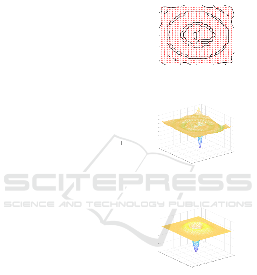
Figure 1: Points in X : only one point (0.1846,0) (marked
x) in the set X
−
with equality constraint v
0
(x,y) = −1 while
the other points (marked ◦) in the set X
0
satisfy inequality
constraints v
0
(x,y) ≤ 0. Moreover, the level set v
0
(x,y) = 0
is shown, approximating the chain-recurrent set.
-1.2
-1
-0.8
1
-0.6
1.5
-0.4
0.5
v'(x,y)
-0.2
1
0
y
0
0.5
0.2
x
0
0.4
-0.5
-0.5
-1
-1
-1.5
Figure 2: The orbital derivative v
0
(x,y) of the constructed
complete Lyapunov function v. v
0
is approximately zero on
the chain-recurrent set (origin and the two periodic orbits,
spheres with radius 0.5 and 1, respectively) and negative ev-
erywhere else. Note that v
0
(0.1846,0) = −1 by the equality
constraint.
-1.5
-1
1
1.5
-0.5
0.5
v(x,y)
1
0
y
0
0.5
x
0
0.5
-0.5
-0.5
-1
-1
-1.5
Figure 3: The constructed complete Lyapunov function
v(x,y). v has a minimum at the asymptotically stable equi-
librium at the origin, a maximum at the unstable periodic
orbit (sphere of radius 0.5) and a minimum at the asymptot-
ically stable periodic orbit (sphere of radius 1).
6 EXAMPLES
6.1 Two Periodic Orbits
We consider the system

˙x
˙y

=

−x(x
2
+ y
2
− 1/4)(x
2
+ y
2
− 1) − y
−y(x
2
+ y
2
− 1/4)(x
2
+ y
2
− 1) + x

.
(23)
Construction of a Complete Lyapunov Function using Quadratic Programming
565

0.01
0.01
0.01
0.01
0.01
0.01
0.01
0.01
0.01
0.01
-0.001
-0.001
-0.001
-0.001
-0.001
-0.001
-0.001
-0.001
-0.001
-0.001
-0.001
-0.001
-0.001
-0.001
-0.001
-0.001
0.01
0.01
0.01
0.01
0.01
0.01
0.01
0.01
0.01
0.01
-0.001
-0.001
-0.001
-0.001
-0.001
-0.001
-0.001
-0.001
-0.001
-0.001
-0.001
-0.001
-0.001
-0.001
-0.001
-0.001
-1 -0.5 0 0.5 1
x
-1
-0.5
0
0.5
1
y
Figure 4: Level sets of the constructed complete Lya-
punov function v(x,y) with level 0.01 (black, maximum)
and −0.001 (red, minimum). This shows that v has a maxi-
mum at the unstable periodic orbit of radius 0.5 and a min-
imum at the asymptotically stable periodic orbit of radius
1.
This system has an asymptotically stable equilib-
rium at the origin as well as two periodic orbits: an
asymptotically stable periodic orbit at Ω
1
= {(x,y) ∈
R
2
| x
2
+ y
2
= 1} and a repelling periodic orbit at
Ω
2
= {(x,y) ∈ R
2
| x
2
+ y
2
= (0.5)
2
}.
For the quadratic programming we have used the
points X =

1.2
13
Z
2
∩ [−1.2,1.2]

\ {(0, 0)} consisting
of 728 points, excluding the equilibrium, and split
them into X
−
= {(0.1846, 0)} (M = 1 point) and X
0
=
X \X
−
(N = 727 points). We have used the Wendland
function ψ
0
(r) = φ
6,4
(r) = (1 − r)
6
+
(35r
2
+ 18r +3).
Figure 1 shows the points marked with a circle
(X
0
) and a cross (X
−
) as well as the level set of
v
0
(x,y) = 0, where v is the constructed complete Lya-
punov function. Figure 2 displays the orbital deriva-
tive v
0
which is −1 at the point (0.1846, 0) and ap-
proximately zero on the equilibrium and the two pe-
riodic orbits (spheres of radius 0.5 and 1). Figure 3
shows the constructed complete Lyapunov function
with a minimum at the origin, which is an asymptot-
ically stable equilibrium, a maximum at the unstable
periodic orbit (sphere of radius 0.5) and a minimum at
the attracting periodic orbit (sphere of radius 1). The
latter minimum can be better seen in Figure 4, where
some level sets of v are displayed.
Note that it is surprising to detect the periodic or-
bit with radius 1, although the only point where we
set the orbital derivative to be −1 is inside circle with
radius 0.5, bounded by the unstable periodic orbit.
A complete Lyapunov function could have been con-
stant on {(x, y) ∈ R
2
|
p
x
2
+ y
2
≥ 0.5}, but this is not
the minimizing solution.
Compared to previous constructions of complete
Lyapunov functions for this example, see (Arg
´
aez
et al., 2017, §4.1) and (Arg
´
aez et al., 2018a, §2.1),
the new method manages to construct a complete Lya-
punov function using only 728 collocation points that
compares favorably with a complete Lyapunov func-
tion that is constructed by solving a system of linear
equations using 29,440 collocation points.
6.2 Homoclinic Orbit
We consider the system
˙
x = f(x), where f(x, y) is
given by

x(1 − x
2
− y
2
) − y((x − 1)
2
+ (x
2
+ y
2
− 1)
2
)
y(1 − x
2
− y
2
) + x((x − 1)
2
+ (x
2
+ y
2
− 1)
2
)

.
(24)
The origin is an unstable focus and the system has
an asymptotically stable homoclinic orbit at a circle
centered at the origin and with radius 1, connecting
the equilibrium (1,0) with itself.
For the optimization we have used the points
X =

1.2
13
Z
2
∩ [−1.2,1.2]

\ {(0,0)} consisting of 728
points, excluding the two equilibria and split them
into X
−
= {(0.1846,0)} (M = 1 point) and X
0
=
X \X
−
(N = 727 points). We have used the Wendland
function ψ
0
(r) = φ
6,4
(r) = (1 − r)
6
+
(35r
2
+ 18r +3).
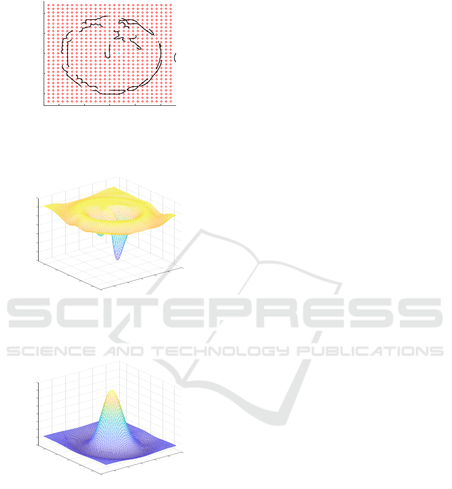
Figure 5 shows the points marked with a circle
(X
0
) and a cross (X
−
) as well as the level set of
v
0
(x,y) = −0.0001, where v is the constructed com-
plete Lyapunov function. Figure 6 displays the orbital
derivative v
0
which is −1 at the point (0.1846,0) and
approximately zero on the homoclinic orbit and the
equilibrium at the origin. Figure 7 shows the con-
structed complete Lyapunov function with a maxi-
mum at the origin and a minimum at the homoclinic
orbit, which is attractive.
Again our novel method compares favorably to
solving a system linear equations using almost 20
times more collocation points, see (Arg
´
aez et al.,
2017, §4.3) and (Arg
´
aez et al., 2018a, §2.3), where
a complete Lyapunov function that is constructed by
solving a system linear equations using 29,440 collo-
cation points.
7 CONCLUSIONS
In this paper we have introduced a new method to con-
struct complete Lyapunov functions. Complete Lya-
punov functions characterize the complete dynamics
of a dynamical system by separating the state space
into the part of the gradient-like flow and the chain-
recurrent set. A complete Lyapunov function has a
strictly negative orbital derivative in the gradient-like
part, while the orbital derivative is zero in the chain-
recurrent set.
For the construction method, one point in the
gradient-like set is chosen, where the orbital deriva-
CTDE 2018 - Special Session on Control Theory and Differential Equations
566

-1 -0.5 0 0.5 1
x
-1
-0.5
0
0.5
1
y
-0.0001
-0.0001
-0.0001
-0.0001
-0.0001
-0.0001
-0.0001
-0.0001
-0.0001
-0.0001
-0.0001
-0.0001
-0.0001
-0.0001
Figure 5: Points in X : only one point (0.1846,0) (marked
x) in the set X
−
with equality constraint v
0
(x,y) = −1 while
the other points (marked ◦) in the set X
0
satisfy inequality
constraints v
0
(x,y) ≤ 0. Moreover, the level set v
0
(x,y) =
−0.0001 is shown, approximating the chain-recurrent set.
-1.2
-1
1
-0.8
-0.6
1.5
0.5
v'(x,y)
-0.4
1
-0.2
y
0
0.5
0
x
0
0.2
-0.5
-0.5
-1
-1
-1.5
Figure 6: The orbital derivative v
0
(x,y) of the constructed
complete Lyapunov function v. v
0
is approximately zero
on the chain-recurrent set (origin and homoclinic orbit) and
negative everywhere else. Note that v
0
(0.1846,0) = −1 by
the equality constraint.
-0.1
0
0.1
1
0.2
1.5
0.3
0.5
v(x,y)
0.4
1
0.5
y
0
0.5
0.6
x
0
0.7
-0.5
-0.5
-1
-1
-1.5
Figure 7: The constructed complete Lyapunov function
v(x,y). v has a maximum at the unstable equilibrium at the
origin and a minimum at the homoclinic orbit at the unit
sphere.
tive is fixed to be −1, and further points are fixed,
where the orbital derivative is bounded from above
by 0. We have formulated this as a minimizing prob-
lem, searching for a function in a reproducing kernel
Hilbert space, which satisfies one equality and finitely
many inequality constraints. Furthermore, we have
shown that this minimization problem in a reproduc-
ing kernel Hilbert space has a unique solution and
that it is of a specific form which can be computed
as quadratic programming problem. The proposed
method was able to successfully construct complete
Lyapunov functions for two test examples with few
points.
Possible extensions include different distributions
of the points in X between X
−
and X
0
: while previous
methods had all points in X
−
, in this paper X
−
con-
sists of only one point. In future work we will develop
a methodology to split the points between these two
sets and combine it with an iterative method, moving
points between these two sets.
ACKNOWLEDGEMENTS
The research in this paper is supported by the Ice-
landic Research Fund (Rann
´
ıs) grant number 163074-
052, Complete Lyapunov functions: Efficient numer-
ical computation.
REFERENCES
Arg
´
aez, C., Giesl, P., and Hafstein, S. (2017). Analysing
dynamical systems towards computing complete Lya-
punov functions. In Proceedings of the 7th In-
ternational Conference on Simulation and Model-
ing Methodologies, Technologies and Applications,
Madrid, Spain, pages 323–330.
Arg
´
aez, C., Giesl, P., and Hafstein, S. (2018a). Compu-
tational approach for complete Lyapunov functions.
accepted for publication in Springer Proceedings in
Mathematics and Statistics Series 2018.
Arg
´
aez, C., Giesl, P., and Hafstein, S. (2018b). Iter-
ative construction of complete Lyapunov functions.
accepted for publication in Proceedings of the 8th
International Conference on Simulation and Model-
ing Methodologies, Technologies and Applications,
Porto, Portugal.
Ban, H. and Kalies, W. (2006). A computational approach
to Conley’s decomposition theorem. J. Comput. Non-
linear Dynam, 1(4):312–319.
Bj
¨
ornsson, J., Giesl, P., Hafstein, S., Kellett, C., and Li, H.
(2015). Computation of Lyapunov functions for sys-
tems with multiple attractors. Discrete Contin. Dyn.
Syst. Ser. A, 35(9):4019–4039.
Conley, C. (1978). Isolated Invariant Sets and the Morse
Index. CBMS Regional Conference Series no. 38.
American Mathematical Society.
Dellnitz, M., Froyland, G., and Junge, O. (2001). The algo-
rithms behind GAIO – set oriented numerical methods
for dynamical systems. In Ergodic theory, analysis,
and efficient simulation of dynamical systems, pages
145–174, 805–807. Springer, Berlin.
Construction of a Complete Lyapunov Function using Quadratic Programming
567

Giesl, P. (2007). Construction of Global Lyapunov Func-
tions Using Radial Basis Functions. Lecture Notes in
Math. 1904, Springer.
Giesl, P. and Wendland, H. (2007). Meshless collocation:
error estimates with application to Dynamical Sys-
tems. SIAM J. Numer. Anal., 45(4):1723–1741.
Goullet, A., Harker, S., Mischaikow, K., Kalies, W., and
Kasti, D. (2015). Efficient computation of Lyapunov
functions for Morse decompositions. Discrete Contin.
Dyn. Syst., 20(8):2419–2451.
Hurley, M. (1992). Noncompact chain recurrence and at-
traction. Proc. Amer. Math. Soc., 115:1139–1148.
Hurley, M. (1998). Lyapunov functions and attractors
in arbitrary metric spaces. Proc. Amer. Math. Soc.,
126:245–256.
Kalies, W., Mischaikow, K., and VanderVorst, R. (2005).
An algorithmic approach to chain recurrence. Found.
Comput. Math, 5(4):409–449.
Narcowich, F. J., Ward, J. D., and Wendland, H. (2005).
Sobolev bounds on functions with scattered zeros,
with applications to radial basis function surface fit-
ting. Mathematics of Computation, 74:743–763.
Schaback, R. and Werner, J. (2006). Linearly constrained
reconstruction of functions by kernels with applica-
tions to machine learning. Adv. Comput. Math., 25(1-
3):237–258.
Wendland, H. (1995). Piecewise polynomial, positive defi-
nite and compactly supported radial functions of min-
imal degree. Adv. Comput. Math., 4(4):389–396.
Wendland, H. (1998). Error estimates for interpolation by
compactly supported Radial Basis Functions of mini-
mal degree. J. Approx. Theory, 93:258–272.
Wendland, H. (2005). Scattered data approximation, vol-
ume 17 of Cambridge Monographs on Applied and
Computational Mathematics. Cambridge University
Press, Cambridge.
CTDE 2018 - Special Session on Control Theory and Differential Equations
568