
Combination of Refinement and Verification for the Construction of
Lyapunov Functions using Radial Basis Functions
Peter Giesl
1
and Najla Mohammed
2
1
Department of Mathematics, University of Sussex, Falmer, BN1 9QH, U.K.
2
Department of Mathematical Sciences, Umm Al-Qura University, Makkah, Saudi Arabia
Keywords:
Lyapunov Function, Domain of Attraction, Radial Basis Function, Refinement Algorithm, Verification
Estimates.
Abstract:
Lyapunov functions are an important tool for the determination of the domain of attraction of an equilibrium
point of a given ordinary differential equation. The Radial Basis Functions collocation method is one of the
numerical methods to construct Lyapunov functions. This method has been improved by combining it with a
refinement algorithm to reduce the number of collocation points required in the construction process, as well
as a verification that the constructed function is a Lyapunov function. In this paper, we propose a combination
of both methods in one, called the combination method. This method constructs a Lyapunov function with the
refinement algorithm and then verifies its properties rigorously. The method is illustrated with examples.
1 INTRODUCTION
In the field of dynamical systems, the domain of at-
traction of an equilibrium is of great importance in
the analysis and the derivation of a dynamical sys-
tem. However, the analytical determination of the
domain of attraction is difficult, therefore researchers
have been seeking numerical algorithms to determine
subsets of the domain of attraction. Most of these are
based on Lyapunov functions, i.e. scalar-valued func-
tions that decrease along trajectories of the dynamical
system.
The existence of a Lyapunov function guarantees
the stability of an equilibrium. Moreover, sublevel
sets of a Lyapunov function are positively invariant
subsets of the domain of attraction. The construction
of such functions, however, is very challenging. For a
review of the numerical methods that have been devel-
oped to construct Lyapunov function, see (Giesl and
Hafstein, 2015).
In this paper we consider an established numerical
method to construct Lyapunov functions using the Ra-
dial Basis Functions (RBF) collocation method. This
method approximates the solution of linear partial dif-
ferential equations (PDEs) using scattered collocation
points and one of its applications is the construction
of Lyapunov functions. More precisely, it considers
a particular Lyapunov function that satisfies a PDE
for its orbital derivatives, and approximately solves
it using meshfree collocation (Giesl, 2007; Giesl and
Wendland, 2007). It turns out that the RBF approxi-
mant itself is a Lyapunov function.
Recently, the construction of Lyapunov functions
using Radial Basis Functions has been improved in
two directions: firstly, the first refinement algorithm
for this method based on Voronoi diagrams has been
proposed in (Mohammed and Giesl, 2015). Starting
with a coarse grid and applying the refinement al-
gorithm the number of collocation points needed to
construct Lyapunov functions has been significantly
reduced. Secondly, a method to rigorously verify
whether the constructed function is a Lyapunov func-
tion, i.e., has negative orbital derivative over a given
compact set, has been proposed in (Giesl and Mo-
hammed, 2018). It uses the specific form of the ap-
proximant and Taylor-type estimates in terms of the
first and second derivatives of the orbital derivative.
In this paper, we will present a combination of
these two methods, i.e., the refinement algorithm and
the verification process, and apply it to examples. The
methodology works in any dimension, however, the
number of collocation points as well as the number of
point evaluations for the verification grows exponen-
tially with the dimension. The refinement algorithm
manages to reduce the number of collocation points.
The outline of this paper will be as follows: Sec-
tion 2 gives the necessary background on dynamical
systems and Lyapunov functions. In Section 3, we
Giesl, P. and Mohammed, N.
Combination of Refinement and Verification for the Construction of Lyapunov Functions using Radial Basis Functions.
DOI: 10.5220/0006944405690578
In Proceedings of the 15th International Conference on Informatics in Control, Automation and Robotics (ICINCO 2018) - Volume 1, pages 569-578
ISBN: 978-989-758-321-6
Copyright © 2018 by SCITEPRESS – Science and Technology Publications, Lda. All rights reserved
569

introduce the construction method of Lyapunov func-
tions using Radial Basis Functions. Section 4 presents
the refinement algorithm and in Section 5 we intro-
duce the verification estimates. Finally, in Section 6,
we propose the new combination method and illus-
trate it with numerical examples before we conclude
in Section 7.
2 LYAPUNOV FUNCTIONS
Consider the following autonomous system of differ-
ential equations
˙x = f (x) (1)
where f ∈C
σ
(R
d
,R
d
), σ ≥ 1 and d ∈ N. We denote
by S
t
ξ := x(t) the solution of the initial value prob-
lem ˙x = f (x), x(0) = ξ ∈ R
d
and we assume that the
solution exists for all t ≥ 0. Note that S
t
defines a
dynamical system on R
d
.
A point x
0
∈R
d
is an equilibrium of (1) if f (x
0
) =
0. Then, x(t) = x
0
for all t ≥ 0 is a constant solution
of (1). The stability of an equilibrium is determined
by the behaviour of solutions in a neighborhood of
an equilibrium. An equilibrium is called stable, if all
solutions starting near the equilibrium stay near the
equilibrium for all future times. Moreover, it is called
asymptotically stable if it is stable and the solutions
starting near the equilibrium converge to it as time
tends to infinity. It is called exponentially stable, if
the rate of convergence to the equilibrium is exponen-
tial. For an asymptotically stable equilibrium x
0
we
are interested in finding the largest set of initial states
from which the trajectories of solutions converge to
the equilibrium as time tends to infinity. This set is
called the domain of attraction.
Definition 1 (Domain of attraction). The domain of
attraction of an asymptotically stable equilibrium x
0
is defined by
A(x
0
) :=
n
x ∈R
d
|S
t
x
t→∞
−→ x
0
o
. (2)
Remark 1. The domain of attraction A(x
0
) of an
asymptotically stable equilibrium x
0
is non-empty and
open.
2.1 Lyapunov Functions
The method of Lyapunov functions enables us to de-
termine subsets of the domain of attraction of an
asymptotically stable equilibrium through sublevel
sets of the Lyapunov function. A function V ∈
C
1
(R
d
,R) is called a (strict) Lyapunov function for
the equilibrium x
0
if it has a local minimum at x
0
and
a negative orbital derivative in a neighborhood of x
0
.
Definition 2 (Orbital derivative). The orbital deriva-
tive of a function V ∈C
1
(R
d
,R) with respect to (1) at
a point x ∈R
d
is defined by
V
0
(x) = h∇V(x), f (x)i,
where h·,·idenotes the standard scalar product in R
d
.
Remark 2. The orbital derivative is the derivative
along solutions; using the chain rule we have
d
dt
V (S
t
x)
t=0
= h∇V(x), ˙xi = h∇V(x), f (x)i = V
0
(x).
(3)
The following theorem shows how Lyapunov
functions are used to find subsets of the domain of
attraction; note that the requirement of the local min-
imum at x
0
is a consequence of the assumptions. The
theorem states that sublevel sets of a Lyapunov func-
tion are positively invariant subsets of the domain of
attraction, see e.g. (Giesl, 2007, Theorem 2.24).
Theorem 1. Let x
0
∈ R
d
be an equilibrium, V ∈
C
1
(R
d
,R) and K ⊂ R
d
be a compact set with neigh-
bourhood B such that x
0
∈
˚
K, where
˚
K denotes the
interior of K. Moreover, let
1. K =
x ∈ B |V (x) ≤ R
for a R ∈ R, i.e., K is a
sublevel set of V .
2. V
0
(x) < 0 for all x ∈K \{x
0
}, i.e., V is decreasing
along solutions in K \{x
0
}.
Then K ⊂ A(x
0
), K is positively invariant and V is
called a (strict) Lyapunov function.
2.2 Existence of Lyapunov Functions
There are several results on converse theorems, ensur-
ing the existence of Lyapunov functions in different
contexts, e.g. already in 1949 (Massera, 1949); for a
review see (Kellett, 2015). These converse theorems,
however, use the explicit solution of (1) and are thus
often not useful to construct a Lyapunov function ex-
plicitly. We will approximate the Lyapunov function
of the following theorem, see (Giesl, 2007, Theorem
2.46).
Theorem 2. Let x
0
be an exponentially stable equi-
librium of ˙x = f (x) with f ∈C
σ
(R
d
,R
d
), σ ≥ 1.
Then there exists a Lyapunov function V ∈
C
σ
(A(x
0
),R
d
) satisfying
V
0
(x) = −kx −x
0
k
2
for all x ∈A(x
0
).
If sup
x∈A(x
0
)
kf (x)k < ∞, then
K
R
:= {x ∈ A(x
0
) |V (x) ≤ R}
is a compact set in R
d
for all R ∈ R.
Note that we can replace the right-hand side by
other functions, e.g. also with a negative constant,
such as V
0
(x) = −1, however, then the function V is
only defined in A(x
0
) \{x
0
}, see also (Giesl, 2007).
CTDE 2018 - Special Session on Control Theory and Differential Equations
570

3 THE CONSTRUCTION OF
LYAPUNOV FUNCTIONS
USING RBF
Meshfree collocation, in particular by Radial Ba-
sis Functions, is used to approximate multivariate
functions and approximately solve partial differen-
tial equations (Powell, 1992; Buhmann, 2003; Sch-
aback and Wendland, 2006). For a general introduc-
tion to meshfree collocation and reproducing kernel
Hilbert spaces see (Wendland, 2005). For the appli-
cation of RBF to the construction of Lyapunov func-
tions, see (Giesl, 2007), where details for the follow-
ing overview of the method can be found, as well as
(Giesl and Wendland, 2007).
A Radial Basis Function is a real-valued function
whose value depends only on the distance from the
origin i.e., Ψ(x) = ψ(kxk
2
), where k·k
2
denotes the
Euclidean norm in R
d
. There is a one-to-one cor-
respondence between a Radial Basis Function and
its reproducing kernel Hilbert space (RKHS). The
approximate solution of the PDE will be a norm-
minimal interpolant in the RKHS; for more details
about this relation the interested reader is referred to
(Giesl and Wendland, 2007).
Now let us consider a general linear partial differ-
ential equation of the form
Lu = g on Ω ⊂ R
d
, (4)
where L is a linear differential operator of the form
Lu(x) =
∑
|α|≤m
c
α
(x)D
α
u(x). (5)
In our case, the differential operator L will be given
by the orbital derivative of a function V with respect
to system (1), namely
LV (x) := h∇V (x), f (x)i=
d
∑
j=1
f
j
(x)∂
j
V (x) = V
0
(x).
(6)
The operator L in (6) is a first order differential
operator of the form (5) with c
e
j
(x) = f
j
(x).
Let X
N
= {x
1
,x
2
,.. .,x
N
} ⊂ Ω be a set of N pair-
wise distinct points which are no equilibria. Define
Dirac’s delta-operator δ by δ
y
0
g(x) = g(y
0
). Then we
have
(δ
x
k
◦L)
x
V (x) = LV (x
k
) = V
0
(x
k
),
where the superscript x denotes the application of the
operator with respect to the variable x. The approxi-
mant v : R
d
→ R of V will be given by
v(x) =
N
∑
k=1
β
k
(δ
x
k
◦L)
y
Ψ(x −y) (7)
where Ψ(x) is the Radial Basis Function. The coeffi-
cients β
k
are determined by claiming that the interpo-
lation condition
(δ
x
j
◦L)
x
V (x) = (δ
x
j
◦L)
x
v(x)
is satisfied for all collocation points x
j
∈ X
N
, or in
other words that the PDE is satisfied at all points x
j
∈
X
N
. This leads to a linear system for β
Aβ = α. (8)
If the points x
j
are pairwise distinct and no equilibria,
then the symmetric matrix A is positive definite, so
in particular non-singular. Hence, the system has a
unique solution β. The interpolation matrix entries of
A = (a
jk
)
j,k=1,...,N
are given by
a
jk
= (δ
x
j
◦L)
x
(δ
x
k
◦L)
y
Ψ(x −y)
and the right-hand side α = (α
j
)
j=1,...,N
is given by
α
j
= (δ
x
j
◦L)
x
V (x) = LV (x
j
) = V
0
(x
j
).
We choose V to be the Lyapunov function from The-
orem 2 and thus α
j
= V
0
(x
j
) = −kx
0
−x
j
k
2
.
Finally, we calculate the approximant v(x) and its
orbital derivative v
0
(x), using the following formulas,
by evaluating and taking the orbital derivative of (7).
v(x) =
N
∑
k=1
β
k
hx
k
−x, f (x
k
)iψ
1
(kx −x
k
k
2
), (9)
v
0
(x) =
N
∑
k=1
β
k
ψ
2
(kx −x
k
k
2
)hx −x
k
, f (x)i×
hx
k
−x, f (x
k
)i
−ψ
1
(kx −x
k
k
2
)hf (x), f (x
k
)i
, (10)
where ψ
1
and ψ
2
are defined as:
ψ
1
(r) =
d
dr
ψ(r)
r
, for r > 0 (11)
ψ
2
(r) =
d
dr
ψ
1
(r)
r
, for r > 0 (12)
and we assume that ψ
1
and ψ
2
can be continuously
extended to 0.
In the following we use a Wendland function φ
`,k
(Wendland, 1998) as Radial Basis Function. Wend-
land functions are compactly supported Radial Ba-
sis Functions, which are polynomials on their sup-
port. The corresponding RKHS is a Sobolev space
with equivalent norm, and, if the smoothness parame-
ter k, defined below, is sufficiently large, then ψ
1
and
ψ
2
can be continuously extended to 0.
The following error estimate was given in (Giesl
and Wendland, 2007, Corollay 4.11). W
τ
2
(Ω) denotes
the usual Sobolev space on Ω ⊂ R
d
. Note that a sim-
ilar estimate holds for the Lyapunov function satisfy-
ing V
0
(x) = −1 in A(x
0
) \{x
0
}.
Combination of Refinement and Verification for the Construction of Lyapunov Functions using Radial Basis Functions
571

Theorem 3. Let k ∈ N if d is odd or k ∈ N \{1} if
d is even and fix ` := b
d
2
c+ k + 1; we use the Radial
Basis Function ψ(r) = φ
`,k
(cr) with c > 0, where φ
`,k
denotes the Wendland function. Set τ = k + (d + 1)/2
and σ = dτe.
Consider the dynamical system defined by (1),
where f ∈ C
σ
(R
d
,R
d
). Let x
0
be an exponentially
stable equilibrium of (1). Let f be bounded in A(x
0
)
and denote by V ∈W
τ
2
(A(x
0
),R) the Lyapunov func-
tion satisfying V
0
(x) = −kx −x
0
k
2
2
. Let Ω ⊂ A(x
0
) be
a bounded domain with Lipschitz continuous bound-
ary.
The reconstruction v of the Lyapunov function V
with respect to the operator (6) and a set X
N
⊂ Ω \
{x
0
} satisfies
kv
0
−V
0
k
L
∞
(Ω)
≤Ch
k−
1
2
kV k
W
k+(d+1)/2
2
(Ω)
(13)
where h := sup
x∈Ω
min
x
j
∈X
N
kx −x
j
k
2
denotes the fill
distance.
Remark 3. If the collocation points are sufficiently
dense, then the right-hand of the error estimate (13)
is smaller than a given ε > 0. This implies that
v
0
(x) ≤V
0
(x) + ε ≤ −kx −x
0
k
2
+ ε < 0
for all x ∈ Ω \B
√
ε
(x
0
). Hence, v has negative or-
bital derivative in Ω apart from a small neighborhood
of x
0
. One can use the Lyapunov function of the lin-
earized system, the so-called local Lyapunov function,
to deal with this small neighborhood of x
0
, for details
see (Giesl, 2007), or a modified method, see (Giesl,
2008). In this paper, we will not deal with this local
problem in more detail, but we exclude a small neigh-
borhood E ⊃ B
√
ε
(x
0
) of x
0
in our consideration.
The error estimate in Theorem 3 establishes that
by choosing the collocation points sufficiently dense,
we will construct a Lyapunov function. However,
there remain two questions: firstly, how do we choose
the collocation points to achieve a negative orbital
derivative with as few collocation points as possible?
The error estimate only gives information about the
error to V
0
based on the fill distance. We, however,
only require v
0
to be negative, so the error could be
larger further away from the equilibrium. The advan-
tage of meshfree collocation is to be able to use scat-
tered points, so it is natural to start with a coarse grid
and introduce a refinement algorithm, see Section 4.
Secondly, the quantities on the right-hand side of
(13) are not explicitly computable, so it remains to
show, after having obtained an approximation v, that
v
0
(x) is negative for all x. This will be done in Section
5.
4 THE REFINEMENT
ALGORITHM
In this section, we will combine the construction
method with a grid refinement algorithm, aiming
for a successful construction of Lyapunov functions
with fewer collocation points and less computation
time than the original method. For more details of
the refinement algorithm see (Mohammed and Giesl,
2015).
Our proposed algorithm is iterative and uses
Voronoi diagrams. In each step, given a set of colloca-
tion points, we generate a Voronoi diagram for these
points. Then, we run a test on each Voronoi vertex
and decide whether we add it to the set of collocation
points or not. A point is added if the orbital derivative
is non-negative.
We have used Voronoi vertices as potential new
collocation points since they are equidistant to three
or more previous grid points, and thus lie “in be-
tween” the grid points. Hence, we avoid collocation
points too close to each other, which would result in a
(nearly) singular interpolation matrix A of the linear
system (8).
4.1 Voronoi Diagrams
A Voronoi diagram is a geometric structure that di-
vides a d-dimensional space into cells based on the
distance between sets of points in the space (Preparata
and Shamos, 1985). Many algorithms for computing
Voronoi diagrams have been proposed, however, we
are going to explain the structure of Voronoi diagrams
via a very simple but less efficient algorithm using
perpendicular hyperplanes.
Let S = {s
1
,s
2
,.. .,s
n
} ⊂ R
d
be a set of n arbi-
trarily distributed and distinct sites (points) in R
d
.
The perpendicular bisector algorithm works as fol-
lows: for each pair of sites in S we construct a hy-
perplane perpendicular to the line segment joining
these sites, which intersects the line segment in the
middle. At the end of this process, we will have in-
tersections of finitely many hyperplanes which build
up cells, with a convex polygon structure, known as
Voronoi regions. The boundaries of each region are
called Voronoi edges and the intersections of Voronoi
edges are called Voronoi vertices. For more details
see (Berg et al., 2008; Klein, 1989; Iyengar et al.,
2014).
Mathematically, the Voronoi region of a point s
i
in
S is defined by
V
i
=
n
\
j=1, j6=i
n
x ∈R
d
|kx −s
i
k
2
< kx −s
j
k
2
o
,
CTDE 2018 - Special Session on Control Theory and Differential Equations
572

where k · k
2
denotes the Euclidean distance. This
means that for every point x ∈ R
d
within a Voronoi
region V
i
the Euclidean distance of x to the site s
i
,
which is also inside the region, is smaller than the Eu-
clidean distance of x to any other site s
j
.
4.2 The Refinement Algorithm
1. Fix a compact neighbourhood K ⊂R
d
and a small
neighborhood E ⊂ K of the equilibrium x
0
as
well as a Radial Basis Function. Let n = 1 and
start with an initial set of collocation points X
1
=
{x
(1)
1
,x
(1)
2
,.. .,x
(1)
N
1
} ⊂ K, not containing any equi-
librium.
2. Calculate a Lyapunov function v
n
using the
RBF method with the collocation points X
n
=
{x
(n)
1
,x
(n)
2
,.. .,x
(n)
N
n
}.
3. Generate Voronoi vertices Y
n
=
{y
1
,y
2
,.. .,y
M
n
} ⊂ R
d
for the collocation points
X
n
. Exclude points in Y
n
which are equilibria, lie
in E or outside K.
4. Run a test on each point y
j
∈Y
n
and check whether
v
0
n
(y
j
) < 0 (then y
j
∈Y
−
n
) or v
0
n
(y
j
) ≥ 0 (then y
j
∈
Y
+
n
), where j = 1, ... ,M
n
and Y
n
= Y
−
n
∪Y
+
n
.
5. Define a new set of collocation points X
n+1
= X
n
∪
Y
+
n
.
6. n → n + 1, repeat the steps 2. to 5. until Y
+
n
=
/
0.
Note that Y
+
n
is the set of Voronoi vertices where the
orbital derivative is non-negative, so they are added to
the set of collocation points, while the orbital deriva-
tive at the vertices Y
−
is already negative.
The algorithm terminates if all Voronoi vertices
have negative orbital derivative. However, this does
not guarantee that the constructed function v
n
has neg-
ative orbital derivative everywhere. In (Mohammed
and Giesl, 2015) the orbital derivative was checked
on a very fine grid, but again, this does not rigorously
show that it is negative everywhere. Hence, in this pa-
per, we will combine this refinement method with the
verification estimates, which will be introduced in the
next section.
5 THE VERIFICATION
ESTIMATES
The motivation of deriving the verification estimates
for the RBF construction method is that the con-
structed function v can not be guaranteed to have neg-
ative orbital derivative in the whole set K. Accord-
ing to the error estimate (13), the approximant v is a
Lyapunov function, if the collocation points are suf-
ficiently dense. However, we can not tell in advance
how small the fill distance h should be since this error
estimate depends on unknown quantities such as V .
Therefore, verification estimates that are based on a
Taylor approximation and rely on the first and second
derivatives of the orbital derivative have been intro-
duced in (Giesl and Mohammed, 2018). They make
use of the special form of the RBF approximant and
its orbital derivative (9) and (10), respectively. The
other main ingredient of these verification estimates
is a checking grid Y
od
. Here, we will only introduce
the verification estimates based on the second deriva-
tives.
In the following we consider two point sets:
1. X
N
= {x
1
,x
2
,.. .,x
N
}, the collocation points for
the calculation of the approximant v.
2. Y
od
= {y
1
,y
2
,.. .,y
M
}, used to check the sign and
value of the orbital derivative of the constructed
Lyapunov function on a different (usually finer but
not necessarily) grid than X
N
.
The checking grid Y
od
consists of vertices of a
fixed triangulation. In (Giesl and Mohammed, 2018)
different triangulations and thus distructions of points
in Y
od
have been considered and it turned out that, de-
pending on whether the dimension d is odd or even,
the standard or the centered triangulation are prefer-
able, i.e. result in fewer points in Y
od
. In this paper
we focus on even dimensions and thus use the stan-
dard triangulation, for odd dimensions see (Giesl and
Mohammed, 2018).
We will introduce triangulations and define the
standard triangulation.
Definition 3. A k-simplex is a set
co(x
0
,.. .,x
k
) =
(
k
∑
i=0
λ
i
x
i
| 0 ≤ λ
i
,
k
∑
i=0
λ
i
= 1
)
,
where x
0
,.. .,x
k
∈ R
d
are pairwise distinct and are
called the vertices.
A triangulation in R
d
is a set T := {T
ν
: ν =
1,2,..., N} (or N = ∞) of d-simplices T
ν
, such that
any two simplices in T intersect in a common face or
are disjoint. Note that a face of a d-simplex is a k-
simplex, 0 ≤ k < d, so this means that the intersection
of two simplices in T is either empty or the convex
combinations of the common vertices of the two sim-
plices.
We denote the set of all vertices of all simplices by
V
T
and we say that T is a triangulation of the set
D
T
:=
[
ν
T
ν
.
Combination of Refinement and Verification for the Construction of Lyapunov Functions using Radial Basis Functions
573

The standard triangulation T
S
(h
1
) with parameter
h
1
∈ R
+
consists of the simplices
T
zJ σ
:= co
x
zJ σ
0
,x
zJ σ
1
,.. .,x
zJ σ
d
for all z ∈ N
d
0
, all J ⊂ {1, 2,... ,d}, and all σ ∈ S
d
,
where
x
zJ σ
i
:= R
J
z +
i
∑
j=1
e
σ( j)
h
1
for i = 0, 1, 2,...,d.
(14)
Here, S
d
denotes the set of all permutations of the
numbers 1,2,... , d and e
1
,e
2
,.. .,e
d
denotes the stan-
dard orthonormal basis of R
d
. Further, the functions
R
J
: R
d
→ R
d
are defined for every J ⊂ {1,2, ..., d}
by
R
J
(x) :=
d
∑
i=1
(−1)
X
J
(i)
x
i
e
i
,
where the characteristic function X
J
(i) is equal to one
if i ∈ J and equal to zero if i /∈ J . Hence, R
J
(x) puts
a minus in front of the coordinates x
i
of x whenever
i ∈ J .
Note that the set of all vertices of all simplices
of the standard triangulation is V
T
S
(h
1
)
= h
1
Z
d
. We
cite Theorem 11 of (Giesl and Mohammed, 2018) and
focus on even dimensions d; note that the theorem
also holds for bounded sets C.
Theorem 4. Let C ⊂ R
d
be a bounded set, v ∈
C
3
(R
d
,R) and f ∈ C
2
(R
d
,R
d
). For d even let T =
{T
ν
∈ T
S
(h
1
) | T
ν
⊂C}, i.e. the simplices of the stan-
dard triangulation with side length h
1
that are fully
contained in C. Let Y
od
= V
T
⊂ h
1
Z
d
and
˜
C = D
T
.
Then
˜
C ⊂C and
v
0
(x) ≤ max
y∈Y
od
v
0
(y) +
d
2
4
max
x∈
˜
C
max
i, j=1,...,d
∂
2
v
0
(x)
∂x
i
∂x
j
h
2
1
(15)
for all x ∈
˜
C.
To estimate the second derivative of the orbital
derivative in (15) we use the following Theorem 10
from (Giesl and Mohammed, 2018), which makes use
of the special form of the approximant v.
Theorem 5 (The second derivative of the orbital
derivative). Let f ∈ C
2
(R
d
,R
d
) and v ∈ C
3
(R
d
,R)
be an RBF approximant of the form (9) with a Ra-
dial Basis Function ψ ∈C
4
(R
+
0
,R). Let
˜
C ⊂ R
d
be a
compact set and X
N
= {x
1
,.. .,x
N
} ⊂
˜
C be a set of N
pairwise distinct points which are no equilibria.
Then the second derivative of the orbital deriva-
tive v
0
can be bounded by
∂
2
v
0
(x)
∂x
i
∂x
j
≤ β
[Ψ
4,4
+ 6Ψ
3,2
+ 3Ψ
2,0
]F
2
+ [2Ψ
3,3
+ 6Ψ
2,1
]FD
1
+ [Ψ
2,2
+ Ψ
1,0
]FD
2
, (16)
for all x ∈
˜
C and all i, j ∈ {1,... ,d}, where
• F := max
x∈
˜
C
kf (x)k
2
,
• D
1
:= max
x∈
˜
C
max
j∈1,...,d
∂ f (x)
∂x
j
2
,
• D
2
:= max
x∈
˜
C
max
i, j∈1,...,d
∂
2
f (x)
∂x
i
∂x
j
2
,
• Ψ
i,k
:= sup
r∈[0,∞)
|ψ
i
(r)|·r
k
,
• β :=
∑
N
k=1
|β
k
|.
Note that we only need a computer to calculate
β, all other quantities can be computed by hand. Ex-
pressions for Ψ
i,k
for certain Wendland functions are
given in (Giesl and Mohammed, 2018).
6 COMBINATION METHOD
In this section we propose a new method, combining
the refinement and verification methods. This method
will rigorously construct a Lyapunov function with
fewer collocation points than previous methods.
Fix a small neighborhood E of the equilibrium and
a compact and convex set E ⊂K ⊂R
d
. Set C = K \E.
We first apply the refinement method until no more
points are added. Let X
N
⊂C be the set of grid points
obtained after the refinement process. Then, the steps
of the combination method are:
1. Calculate the quantities F,D
1
,D
2
,Ψ
i,k
,β, and sub-
stitute in (16).
2. Use estimate (15) to determine the order of h
1
,
i.e., the density of the checking grid Y
od
.
3. Use this h
1
to define Y
od
and calculate the maxi-
mum value of the orbital derivative v
0
in Y
od
.
4. Use estimate (15) to show that v
0
(x) < 0 for all
x ∈
˜
C, and thus that the constructed function v is a
Lyapunov function.
5. If 4. fails, then either the initial grid of the refine-
ment or the checking grid is not fine enough.
We will now apply the combination method to two
examples – one where both methods have previously
been applied to in isolation, and one new one.
Example 1. Consider the non-linear system (Giesl
and Wendland, 2007, Example 4.3)
(
˙x = −x −2y + x
3
,
˙y = −y +
1
2
x
2
y + x
3
.
The system has an asymptotically stable equilibrium
at (0, 0) and we have used the refinement algorithm to
construct an approximant v of the Lyapunov function
satisfying V
0
(x) = −kxk
2
2
. In (Mohammed and Giesl,
CTDE 2018 - Special Session on Control Theory and Differential Equations
574
2015), Example 3, the Wendland function φ
6,4
(r) =
(1 −r)
6
+
(35r
2
+ 18r + 3), where x
+
= x for x ≥0 and
x
+
= 0 for x < 0 was used. The refinement process
was started with an initial set X
initial
of 24 colloca-
tion points. The algorithm terminated after four re-
finement steps with the set X
f inal
of 90 collocation
points with K = [−1,1]
2
and E = (−0.1,0.1)
2
. The
sign of v
0
was checked over a checking grid X
check
of
size h
check
= 10
−3
. However, this does not rigorously
show that the function has negative orbital derivative
everywhere.
In (Giesl and Mohammed, 2018), Example 1, the
same example has been considered, but with a regular,
larger set of 360 collocation point. It has been shown,
using the verification estimates, that the constructed
function has negative orbital derivative.
We will now use the combination method in this
paper, again starting with an initial set X
initial
of 24
collocation points. We have used the Wendland func-
tion φ
6,4
and K = [−1, 1]
2
, but have excluded the set
E = [−0.1,0.1]
2
and set C = K \E. The refinement
algorithm terminated after four refinement steps with
the set X
f inal
of N
4
= 88 collocation points, see Figure
1. The time to calculate the four refinement steps on
a standard laptop with an Intel(R) Core (TM) i5-3550
CPU @ 3.30 GHz processor was 2.1 seconds.
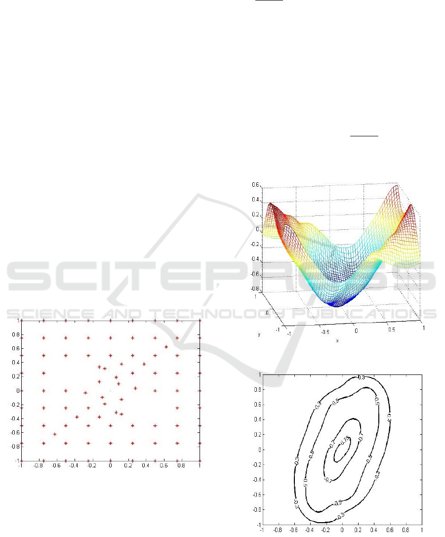
Figure 2 (a) shows the Lyapunov function v
4
con-
structed with the final set of collocation points ob-
tained with the refinement algorithm. Figure 2 (b),
displays different sublevel sets of v
4
.
Figure 1: The grid points N
4
= 88 after the termination of
the refinement algorithm.
We continue with the verification of the obtained
Lyapunov function. We will derive and then use an
estimate for the size of the checking grid to verify the
negativity of the orbital derivative of v.
We have F = 4.717, D
1
= 5.657, and D
2
=
9.2195. We calculate the value of β =
∑
88
k=1
|β
k
| =
0.4105.
Hence, (16) gives
∂
2
v
0
(x)
∂x
i
∂x
j
≤ 0.4105
157870.623 ×(4.717)
2
+ 19358.745 ×4.717 ×5.657
+ 1124.797 ×4.717 ×9.2195
= 1.7 ×10
6
. (17)
Since d = 2 is even, we use Theorem 4 and use the
estimate (17) in (15). We obtain
v
0
(x) ≤ max
y∈Y
od
v
0
(y)
+
max
x∈
˜
C
max
r,s=1,2
∂
2
v
0
(x)
∂x
r
∂x
s
h
2
1
,
≤ max
y∈Y
od
v
0
(y) +
1.7 ×10
6
h
2
1
. (18)
(a) The constructed Lyapunov function v
4
(x,y)
with the refinement algorithm.
(b) Different sublevel sets of v
4
.
Figure 2: (a) The constructed Lyapunov function v
4
(x,y)
with the refinement algorithm and (b) different sublevel sets
of v
4
.
Combination of Refinement and Verification for the Construction of Lyapunov Functions using Radial Basis Functions
575
Assume that the orbital derivative of the con-
structed function v
0
is a good approximation to V
0
with V
0
(x) = −kxk
2
2
in [−1,1]
2
\[−0.1,0.1]
2
. Then
sup
y∈[−1,1]
2
\[−0.1,0.1]
2
v
0
(y) ≈ −0.1
2
.
The right-hand side of (18) is negative if
1.7 ×10
6
h
2
1
≤ 10
−2
h
1
≤
r
1
1.7
10
−4
= 7.67 ·10
−5
.
The estimated value of h
1
indicates the supposed den-
sity of the checking grid Y
od
. To allow for a small er-
ror, we have chosen the density of Y
od
to be h
1
= 4.17 ·
10
−5
. Then checking the value of the orbital deriva-
tive over Y
od
= h
1
Z
2
∩C gives max
y∈Y
od
v
0
(y) = −0.0038.
These function evaluations took 47,290.4 seconds on
the same laptop, note that this could be parallelized
to make the computation faster. Therefore, (18) yields
v
0
(x) ≤ −0.0038 +
1.7 ×10
6
4.17 ×10
−5
2
,
= −0.0038 + 0.003 = −0.0008,
which shows that v
0
(x) < 0 for all x ∈
˜
C = [−1,1]
2
\
(−0.1 −h
1
,0.1 +h
1
)
2
, i.e. the function v, constructed
by the refinement method, is a Lyapunov function.
Example 2. We will now consider
(
˙x = −x(1 −x
2
−y
2
) −y,
˙y = −y(1 −x
2
−y
2
) + x,
see (Giesl, 2007, Example 2.10), which has an expo-
nentially stable equilibrium at x
0
= (0,0) with domain
of attraction B
1
(0,0). We use the refinement algo-
rithm to construct an approximant v of the Lyapunov
function satisfying V
0
(x) = −1. Note that such a func-
tion exists in A(x
0
) \{x
0
}.
We set K = [−0.9,0.9]
2
, E = [−0.1, 0.1]
2
and
C = K \E. We choose the Wendland function φ
6,4
,
see previous example. We start our refinement algo-
rithm with an initial set of collocation points X
1
=
{(x,y) ∈ R
2
| x,y ∈ {0, ±h,.. .,±0.9}}\E, h = 0.36,
i.e. N
1
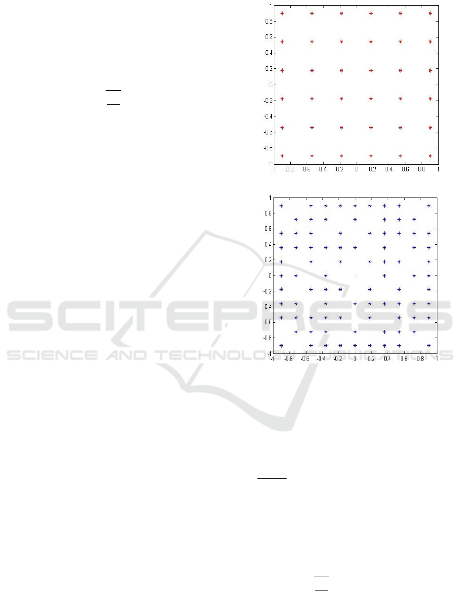
= 36 points, see Figure 3 (a).
After performing four refinement steps, the algo-
rithm terminates and constructs a function v
4
with
N
4
= 88 points, see Figure 3 (b). The time to calculate
the four refinement steps was 1.8 seconds.
Figure 4 (a) shows the Lyapunov function v
4
con-
structed with the final set of collocation points ob-
tained with the refinement algorithm N
4
= 88 points.
Figure 4 (b) displays different sublevel sets of v
4
.
Let us now verify that the constructed function is
indeed a Lyapunov function. We first calculate the
quantities F = 3.57, D
1
= 4.98, D
2
= 5.69 as well as
β =
∑
88
k=1
|β
k
| = 1.7372.
(a) The initial grid X
1
with N
1
= 36 points.
(b) The final grid X
4
with N
4
= 88 points.
Figure 3: (a) shows the distribution the initial grid points
and (b) the distribution of final grid points after the last re-
finement step.
We now use the verification estimates to determine
the order of the checking grid Y
od
. We calculate the
second derivative of the orbital derivative by (16)
∂
2
v
0
(x)
∂x
i
∂x
j
≤ 1.7372 ×2379065.026 = 4.1 ×10
6
.
Since d = 2 is even, we apply Theorem 4. Thus,
v
0
(x) ≤ max
y∈Y
od
v
0
(y) +
4.1 ×10
6
h
2
1
. (19)
If v
0
is a good approximation to V
0
, then max
y∈Y
od
v
0
(y) ≈
−1. The right-hand side of (19) is negative if
h
1
≤
r
1
4.1
10
−3
≈ 0.494 ×10
−3
.
To allow for an error, we have chosen the density
of Y
od
to be h
1
= 4.05 × 10
−5
. Then checking the
value of the orbital derivative over Y
od
= h
1
Z
2
∩C
CTDE 2018 - Special Session on Control Theory and Differential Equations
576
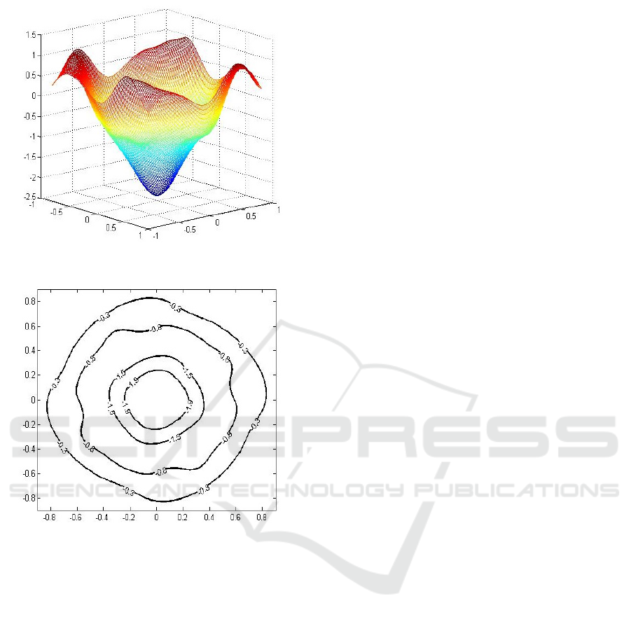
(a) The constructed Lyapunov function v
4
(x,y) with
the refinement algorithm.
(b) Different sublevel sets of v
4
.
Figure 4: (a) The constructed Lyapunov function v
4
(x,y)
with the refinement algorithm and (b) different sublevel sets
of v
4
.
gives max
y∈Y
od
v
0
(y) = −0.0142. These function evalua-
tions took 35,904.5 seconds on the same laptop, note
that this could be parallelized to make the computa-
tion faster. Therefore, (19) yields
v
0
(x) ≤ −0.0142 +
4.1 ×10
6
4.05 ×10
−5
2
,
= −0.0142 + 0.0067 = −0.0075.
Thus, v
0
(x) < 0 for all x ∈
˜
C = [−1, 1]
2
\(−0.1 −
h
1
,0.1+h
1
)
2
, and the constructed function v is a Lya-
punov function.
Note that K is not a subset of the domain of attrac-
tion. As usually the domain of attraction is not known
in advance, this is a realistic situation, and even in
this situation, the algorithm works well.
7 CONCLUSION
Lyapunov functions are an important tool to deter-
mine the domain of attraction of an equilibrium. They
can be constructed by approximating a solution of a
PDE using Radial Basis Functions. This paper com-
bines a refinement algorithm of this method, refin-
ing the set of collocation points using Voronoi ver-
tices, with a verification that the constructed function
is indeed a Lyapunov function. The refinement al-
gorithm results in fewer collocation points than by
uniformly refining the set of collocation points. The
verification provides a rigorous method to show that
the constructed function has a negative orbital deriva-
tive. The combination of these two methods, which
was proposed for the first time in this paper, thus pro-
vides an efficient and rigorous method to construct
Lyapunov functions. This was demonstrated in two
examples.
REFERENCES
Berg, M., Cheong, O., Kerveld, M., and Overmars, M.
(2008). Computational geometry: Algorithms and Ap-
plications. Springer-Verlag, Berlin.
Buhmann, M. (2003). Radial basis functions: theory and
implementations, volume 12 of Cambridge Mono-
graphs on Applied and Computational Mathematics.
Cambridge University Press, Cambridge.
Giesl, P. (2007). Construction of Global Lyapunov Func-
tions Using Radial Basis Functions. Lecture Notes in
Math. 1904, Springer.
Giesl, P. (2008). Construction of a local and global Lya-
punov function using Radial Basis Functions. IMA J.
Appl. Math., 73(5):782–802.
Giesl, P. and Hafstein, S. (2015). Review on computational
methods for Lyapunov functions. Discrete Contin.
Dyn. Syst. Ser. B, 20:2291–2331.
Giesl, P. and Mohammed, N. (2018). Verification esti-
mates for the construction of Lyapunov functions us-
ing meshfree collocation. submitted.
Giesl, P. and Wendland, H. (2007). Meshless collocation:
error estimates with application to Dynamical Sys-
tems. SIAM J. Numer. Anal., 45(4):1723–1741.
Iyengar, S., Boroojeni, K., and Balakrishnan, N. (2014).
Mathematical Theories of Distributed Sensor Net-
works. Springer, New York.
Kellett, C. M. (2015). Classical converse theorems in Lya-
punov’s second method. Discrete Contin. Dyn. Syst.
Ser. B., 20(8):2333–2360.
Klein, R. (1989). Concrete and Abstract Voronoi Diagrams.
Lecture Notes in Computer Science. Springer-Verlag,
Berlin.
Massera, J. (1949). On Liapounoff’s conditions of stability.
Ann. of Math., 50(2):705–721.
Combination of Refinement and Verification for the Construction of Lyapunov Functions using Radial Basis Functions
577

Mohammed, N. and Giesl, P. (2015). Grid refinement in
the construction of Lyapunov functions using radial
basis functions. Discrete Contin. Dyn. Syst. Ser. B,
20:2453–2476.
Powell, M. J. D. (1992). The theory of radial basis func-
tion approximation in 1990. In Advances in numerical
analysis, Vol. II (Lancaster, 1990), Oxford Sci. Publ.,
pages 105–210. Oxford Univ. Press, New York.
Preparata, F. and Shamos, M. (1985). Computational ge-
ometry. Texts and Monographs in Computer Science.
Springer-Verlag, New York.
Schaback, R. and Wendland, H. (2006). Kernel techniques:
from machine learning to meshless methods. Acta Nu-
mer., 15:543–639.
Wendland, H. (1998). Error estimates for interpolation by
compactly supported Radial Basis Functions of mini-
mal degree. J. Approx. Theory, 93:258–272.
Wendland, H. (2005). Scattered data approximation, vol-
ume 17 of Cambridge Monographs on Applied and
Computational Mathematics. Cambridge University
Press, Cambridge.
CTDE 2018 - Special Session on Control Theory and Differential Equations
578
