Verification of a Numerical Solution to a Collocation Problem
Hjortur Bjornsson and Sigurdur Hafstein
Science Institute and Faculty of Physical Sciences, University of Iceland, Dunhagi 5, 107 Reykjav
´
ık, Iceland
Keywords:
Numerical Computation, Lyapunov Function, Radial Basis Functions.
Abstract:
In a recent method to compute Lyapunov functions for nonlinear stochastic differential equations a subsequent
verification of the results is needed. The theory has been developed but there are several practical difficulties in
its implementation because of the huge amount of function evaluations needed during verification. We study
several different methods and compare their accuracy and efficiency.
1 INTRODUCTION
We will discuss numerical solutions to Partial Dif-
ferential Equations (PDE) that arise when computing
Lyapunov functions for Stochastic Differential Equa-
tions (SDE) and, in particular, how the validity of the
computed Lyapunov functions can be verified numer-
ically. In a novel numerical method (Bjornsson et al.,
2018) we obtain a numerical solution to a PDE, and
that solution is supposed to be a Lyapunov function
for a certain SDE. To guarantee that the numerical so-
lution is in fact a Lyapunov function, we have an error
estimate which states that if the value of the numerical
solution on a certain grid of points is lower then some
constant, then the numerical solution is indeed a Lya-
punov function for the system. The theory support-
ing this novel method was developed in (Gudmunds-
son and Hafstein, 2018; Hafstein et al., 2018), and in
(Bjornsson et al., 2018) the method is developed and
it is shown that it converges to a true Lyapunov func-
tion if the collocation grid used for the numerical so-
lution of the PDE is sufficiently dense. However, one
must verify a posteriori on an evaluation grid that the
collocation grid was indeed adequate. An issue with
the method is that the evaluation grid is so dense that
we need to evaluate the computed Lyapunov function
at typically 10
9
, and even up to 10
16
, points. Note
that the Lyapunov function is computed using Radial
Basis Functions (RBF) and to evaluate it at a point,
one must sum over all the RBFs used in the compu-
tation, i.e. the sum contains a number of terms that
is equal to the number of the collocation points used.
Here we will compare the numerical errors and per-
formances of various methods used for this nontrivial
and involved evaluation.
2 BACKGROUND
For completeness we give a quick background with
many of the details omitted. For full details see (Gud-
mundsson and Hafstein, 2018; Hafstein et al., 2018;
Bjornsson et al., 2018). We consider a d-dimensional
SDE of the form
dX(t) = f (X(t))dt + g(X(t))dW (t), (1)
where f : R
d
→ R
d
, g : R
d
→ R
d×Q
, f (0) = g(0) = 0,
and W (t) is a Q-dimensional Brownian motion. We
are specifically interested in the stability of the trivial
solution X = 0 of the system.
Let Ω ⊂ R
d
be a bounded domain with a smooth
boundary Γ = ∂Ω. We solve numerically the bound-
ary problem of the PDE given by:
(
LV (x) = r(x) for x ∈ Ω,
V (x) = c(x) for x ∈ Γ,
(2)
where L denotes the following differential operator
associated with the system given in equation (1):
LV (x) =
1
2
d
∑
i, j=1
m
i j
(x)
∂
2
v
∂x
i
∂x
j
(x) +
d
∑
i=1
f
i
(x)
∂v
∂x
i
(x),
(3)
where (m
i j
(x))
i, j
= g(x)g(x)
>
. For suitable functions
r(x) and c(x) the solution to this PDE will be a Lya-
punov function asserting the asymptotic stability in
probability of the trivial solution and we can use it to
estimate its probabilistic basin of attraction.
To solve this PDE numerically we use the RBF
method similar to (Giesl, 2007; Giesl, 2008; Giesl
and Wendland, 2007), where Lyapunov functions are
computed for deterministic ordinary differential equa-
tions (ODEs), but adapted to SDEs. Given a set
Bjornsson, H. and Hafstein, S.
Verification of a Numerical Solution to a Collocation Problem.
DOI: 10.5220/0006945405870594
In Proceedings of the 15th International Conference on Informatics in Control, Automation and Robotics (ICINCO 2018) - Volume 1, pages 587-594
ISBN: 978-989-758-321-6
Copyright © 2018 by SCITEPRESS – Science and Technology Publications, Lda. All rights reserved
587

of points X
1
= {x
1
,..., x
N
} ⊂ Ω ⊂ R
d
and X
2
=
{ξ
1
,..., ξ
M
} ⊂ Γ, we solve the interpolation problem
(
LV (x
i
) = r(x
i
) for all i = 1, .. ., N,
V (ξ
i
) = c(ξ
i
) for all i = 1, .. ., M.
(4)
The solution to the interpolation problem is given by
V (x) =
N
∑
k=1
α
k
(δ
x
k
◦ L)
y
ψ(kx − yk)
+
M
∑
k=1
α
N+k
(δ
ξ
k
◦ L
0
)
y
ψ(kx − yk)
(5)
where δ
y
V (x) = V (y) and the superscript y denotes
that the operator is applied with respect to the vari-
able y, L
0
= id and ψ = ψ
l,k
is a so-called Wend-
land function, which are compactly supported RBFs
(Wendland, 1998). The constants α
k
in equation (5)
can be determined as the solution to a certain linear
system Aα = γ, where the matrix A is symmetric and
positive definite; see (Bjornsson et al., 2018) for full
details on the matrix A and the vector γ.
2.1 Lyapunov Function
The method described in the preceding section is
used to compute a certain Lyapunov function for
the system (1), whose domain does not include the
equilibrium at the origin, hence the name non-local
Lyapunov function. Again see (Gudmundsson and
Hafstein, 2018; Hafstein et al., 2018; Bjornsson et al.,
2018) for details.
Definition (Non-Local Lyapunov Function). Let
A,B ⊂ R
d
, B ⊂ A
◦
, be simply connected compact
neighbourhoods of the origin with C
2
boundaries
and set U := A \ B
◦
. A function V ∈ C
2
(U) for the
system (1) such that
(1) 0 ≤ V (x) ≤ 1 for all x ∈ U,
(2) LV (x) < 0 for all x ∈ U, and
(3) V
−1
(0) = ∂B and V
−1
(1) = ∂A ,
is called a non-local Lyapunov function for the
system (1), and we refer to ∂B and ∂A is the inner
and outer boundary of U, respectively.
To compute a non-local Lyapunov function for the
system (1) we look for solutions of the PDE (2) with
r(x) = −h where h > 0 is a small constant, c(x) = 1
for x ∈ ∂A and c(x) = 0 for x ∈ ∂B . Because we
compute a numerical approximation to the solution
of the system we can not expect LV (x) = −h to hold
for all x ∈ U, but since the definition of a non-local
Lyapunov function only requires LV (x) < 0, our nu-
merical approximation will still be a true Lyapunov
function as long as there is no point in x ∈ U with
LV (x) ≥ 0. In this paper we are concerned with the
numerical verification of the condition that LV (x) < 0
holds for all x ∈ U. The theory for this verification
is developed in (Bjornsson et al., 2018). Here we are
interested in the nontrivial technical details of its effi-
cient implementation.
2.2 Explicit Formulas
For the explicit computations of our Lyapunov func-
tion, one must choose a specific Wendland function
ψ
k,l
(x), where the indices k,l are non-negative inte-
gers. In the one dimensional case we have used ψ
7,6
and for two dimensional cases we used ψ
8,6
. Note
that there are certain restriction on the indices of the
Wendland function for the problem at hand and in our
computations we need at least these rather large in-
dices.
For example, assuming we are using the Wend-
land function ψ
7,6
and the RBF constant c > 0, we
define by some abuse of notation ψ
0
(r) := ψ
7,6
(cr)
for r ≥ 0. Then we define ψ
i+1
(r) =
1
r
∂
∂r
ψ
i
(r) re-
cursively for i = 0, 1,2, 3. Finally, we define W
i
(x) =
ψ
i
(x/c). The formulas for the functions W
i
starting
with ψ
0
:= ψ
7,6
are the following:
W
0
(x) = (1 −x)
13
(4096x
6
+ 7059x
5
+ 5751x
4
+ 2782x
3
+ 830x
2
+ 143x +11),
(6)
W
1
(x) = − 38c
2
(1 − x)
12
(2048x
5
+ 2697x
4
+ 1644x
3
+ 566x
2
+ 108x +9),
(7)
W
2
(x) = 10336c
4
(1 − x)
11
(128x
4
+ 121x
3
+ 51x
2
+ 11x +1),
(8)
W
3
(x) = − 62016c
6
(1 − x)
10
(320x
3
+ 197x
2
+ 50x +5), and
(9)
W
4
(x) = 3224832c
8
(1 − x)
9
(80x
2
+ 27x +3).
(10)
Note that these formulas are only valid for 0 ≤ x ≤ 1
and for x > 1 we have W
i
(x) = 0. The parameter c is
referred to as the RBF constant and is used to control
the size of the support of the functions R
d
→ R
d
, x 7→
ψ
i
(kxk), i.e. the support is a ball of radius 1/c around
the origin.
The explicit formulas for V (x) and LV (x) from our
numerical solution to the interpolation problem (4),
and by writing β = x −x
k
for brevity, are given by the
CTDE 2018 - Special Session on Control Theory and Differential Equations
588

following expressions:
V (x) =
N
∑
k=1
α
k

− ψ
1
(kβk)hβ, f (x
k
)i
+
1
2
d
∑
i, j=1
m
i j
[ψ
2
(kβk)β
i
β
j
+ δ
i j
ψ
1
(kβk)]

+
M
∑
k=1
α
N+k
ψ
0
(kβk) (11)
and
LV (x)
=
N
∑
k=1
α
k

− ψ
2
(kβk)hβ, f (x)ihβ, f (x
k
)i
− ψ
1
(kβk)h( f (x), f (x
k
))i
+
1
2
d
∑
i, j=1
m
i j
(x
k
)

ψ
3
(kβk)hβ, f (x)iβ
i
β
j
+ ψ
2
(kβk) f
j
(x)β
i
+ ψ
2
(kβk) f
i
(x)β
j
+ δ
i j
ψ
2
(kβk)hβ, f (x)i

+
1
2
d
∑
i, j=1
m
i j
(x)

− ψ
3
(kβk)hβ, f (x
k
)iβ
i
β
j
− ψ
2
(kβk) f
j
(x
k
)β
i
− ψ
2
(kβk) f
i
(x
k
)β
j
− δ
i j
ψ
2
(kβk)hβ, f (x
k
)i

+
1
4
d
∑
r,s=1
d
∑
i, j=1
m
rs
(x)m
i j
(x
k
)

ψ
4
(kβk)β
i
β
j
β
r
β
s
+ ψ
3
(kβk)[δ
i j
β
r
β
s
+ δ
ir
β
j
β
s
+ δ
is
β
j
β
r
+ δ
jr
β
i
β
s
+ δ
js
β
i
β
s
+ δ
rs
β
i
β
j
]
+ ψ
2
(kβk)[δ
i j
δ
rs
+ δ
ir
δ
js
+ δ
is
δ
jr
]

+
M
∑
k=1
α
N+k

− ψ
1
(kξ
k
− xk)hξ
k
− x, f (x)i
+
1
2
d
∑
i, j=1
m
i j
(x)[ψ
2
(kξ
k
− xk)(ξ
k
− x)
i
(ξ
k
− x)
j
+ δ
i j
ψ
1
(kξ
k
− xk)]

. (12)
In these formulas α = (α
1
,α
2
,..., α
N+M
)
>
is the so-
lution to Aα = γ associated with the interpolation
problem (4) and β
i
is the i-th component of the vector
β = x − x
k
. Note the above formulas are independent
of which Wendland function ψ
k,l
we start with in the
beginning.
3 VERIFICATION
Let A ,B , and U be as in the definition of non-local
Lyapunov functions and let V (x) be a numerical ap-
proximation like is described afterwards. Now by
(Bjornsson et al., 2018, Theorem 4.3), if
ν := max
y∈Y
U
LV (y) +C
u
d
2
4
h
2
< 0, (13)
then V is a non-local Lyapunov function for the sys-
tem. Here d is the dimension of the system, h > 0
is a parameter controlling the density of the evalua-
tion grid, and Y
U
is the evaluation grid that covers
U. Finally the constant C
U
is an upper estimate on
the second derivatives of our function LV , for further
details see (Bjornsson et al., 2018; Mohammed and
Giesl, pted).
3.1 One Dimensional Example
For an explicit example let us consider the one dimen-
sional SDE from (Bjornsson et al., 2018)
dx(t) = sin(x(t))dt +
3x(t)
1 + x(t)
2
dW (t), (14)
where W is a one dimensional Brownian motion. We
determine an approximate solution to the PDE:





LV (x) = −10
−3
for 10
−2
< x < 8,
V (x) = 0 for x = 10
−1
,
V (x) = 1 for x = 8.
(15)
The approximate solution was determined using the
Wendland function ψ
7,6
, the RBF constant c = 2, and
700 evenly spaced collocation points on the interval
[1.1 · 10
−2
,7.99]. Figure 1 shows the numerical solu-
tion to PDE (15), for the system in equation (14). For
this system and these values the estimate C
U
is equal
to 1.6846 · 10
12
.
0 1 2 3 4 5 6 7 8
0
0.2
0.4
0.6
0.8
1
1.2
Figure 1: Numerical solution of V(x) in equation (15).
Verification of a Numerical Solution to a Collocation Problem
589

By estimating through rough computations that
the maximum value of our numerical approximation
to LV(x) is 0.3 × 10
−3
, we get by setting ν = 0 in
equation (13)
h =
r
4 · 0.3 · 10
−3
1.6846
= 2.6 ·×10
−8
.
To give us some safety, which is needed since ν has to
be strictly negative, we choose h = 2.18 · 10
−8
. This
corresponds to evaluating the function LV at 7.5 · 10
8
evenly spaced points Y
U
on the interval [10
−2
−h, 8 +
h]. This large number of points that needs to be evalu-
ated takes about 10 seconds on a normal desktop com-
puter (i7 4790k). The maximum value of LV found on
this grid is −0.281 · 10
−3
and thus
ν = −0.281 ·10
−3
+ 0.19119 · 10
−3
< 0,
so our approximation is a non-local Lyapunov func-
tion.
3.2 Two Dimensional Example
For a second explicit example consider the two di-
mensional system from (Gr
¨
une and Camilli, 2003)
also studied in (Bjornsson et al., 2018), given by
dx(t) = (M + ρ(x(t))I)x(t)dt + g(x(t))dW (t), (16)
where W is a one dimensional Brownian motion, I the
2 × 2-identity matrix,
M =

0 1
−1 0

, ρ(x) = kxk − 1,
and
g(x) = kxk

kxk −
1
2

kxk −
3
2

x.
We find an approximate solution to the PDE, LV (x) =
−10
−2
, on an annulus around the origin with inner
radius 0.4 and outer radius 1.9 with V (x) = 0 for
kxk = 0.4 and V (x) = 1 for kxk = 1.9. To calcu-
late the approximation we used the Wendland func-
tion ψ
8,6
and a grid of 80 × 80 points evenly spaced
on the annulus. Figure 2 shows the resulting numer-
ical approximation for the system in equation (16).
For this system, and using ψ
8,6
, the constant C
U
is
determined to be 4.3220 · 10
12
, and following similar
calculations as in the preceding section we estimate
the maximum value of LV to be ≈ −0.005, this gives
us h = 3.4013 · 10
−8
, so we need to evaluate LV on a
grid with (1.1760 · 10
8
)
2
≈ 10
16
points.
3.3 Comparison of Methods
In the inner-most loop of our program we have to
evaluate W
i
, i = 1,2, 3,4. For simplicity we con-
sider only the polynomials resulting from the Wend-
land function ψ
7,6
given by equations (7)-(10) and we
-0.5
2
0
1
2
0.5
1
1
0
1.5
0
-1
-1
-2
-2
Figure 2: Numerical solution of V (x) for the two dimen-
sional system (16).
fixed c = 2; the function (6) is unused as LV does
not depend on it. We tried different Wendland func-
tions but the results were comparable. Fast evaluation
of these functions is critical for the performance of
our verification, therefore we tested 5 different eval-
uation methods: having these functions hardcoded in
factorized form as in (7)-(10), expanding the polyno-
mials and using Horner’s method for the evaluation,
using Lookup-tables, using a Lookup-table and addi-
tionally applying linear interpolation, and combining
the two previous approaches on different subintervals.
All tests were written in C and compiled using gcc
with optimization flag -O2. The figures in the fol-
lowing section only show function (10) since it has
the largest numerical errors. The errors for the other
functions, i.e. (7)-(9), are qualitatively identical but of
lower magnitude.
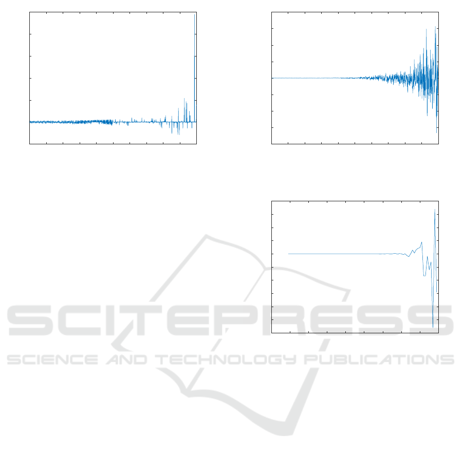
3.3.1 Evaluation with Hardcoded Functions
We hardcoded the polynomials as they are written in
equations (7)-(10).
0 0.1 0.2 0.3 0.4 0.5 0.6 0.7 0.8 0.9 1
-1.5
-1
-0.5
0
0.5
1
1.5
× 10
-6
Figure 3: Absolute error as a function of x of W
4
using Hard-
coded Functions. Note the scale on the y-axis is ×10
−6
.
CTDE 2018 - Special Session on Control Theory and Differential Equations
590

0 0.1 0.2 0.3 0.4 0.5 0.6 0.7 0.8 0.9 1
-1
0
1
2
3
4
5
× 10
-14
Figure 4: Relative error as a function of x of W
4
using Hard-
coded Functions. Note the scale on the y-axis is ×10
−14
.
Figures 3 and 4 show the absolute and relative
error, respectively, of the function W
4
compared to
the values obtained from infinite precision arithmetic
truncated to 64-bit floating point values. These fig-
ures show us that this method, i.e. having hardcoded
functions, gives us the best accuracy out of all of the
methods tested.
3.3.2 Evaluation using Horner’s Method
We expanded the polynomials, i.e. obtained coeffi-
cients a
n
,a
n−1
,..., a
0
such that
W
i
(x) = a
n
x
n
+ a
n−1
x
n−1
+ ·· · + a
0
.
Obviously the coefficients a
i
depend on which Wend-
land function ψ
k,l
we started with. Having the poly-
nomials in expanded form allows us to evaluate them
at any point x using the following scheme (Horner’s
method):
Horner(x, [a_n])
acc:=0;
for(i=n;i>=0;i--)
acc=acc*x;
acc=acc+a_i;
return acc;
By taking advantage of SIMD-instructions (Sin-
gle Instruction, Multiple Data) we can evaluate two of
these polynomials at a time in double precision arith-
metic, or even all four at the same time on machines
that support 256-bit wide SIMD registers (AVX2 or
later).
Since the polynomial functions have a high or-
der zero at x = 1, and the coefficients are relatively
large, we get significant absolute errors in the evalua-
tion when x is close to 1, see figure 5. For the func-
tion W
4
the relative error close to x = 1 explodes, as
the value of the function is close to 0 there. Using
higher values for the Wendland RBF constant c exag-
gerates this behaviour, so it is virtually impossible to
0 0.1 0.2 0.3 0.4 0.5 0.6 0.7 0.8 0.9 1
-8
-6
-4
-2
0
2
4
6
8
× 10
-4
Figure 5: Absolute error as a function of x of W
4
using
Horner’s method. Note the scale on the y-axis is ×10
−4
.
0.89 0.9 0.91 0.92 0.93 0.94 0.95 0.96 0.97 0.98
-1.2
-1
-0.8
-0.6
-0.4
-0.2
0
0.2
0.4
0.6
0.8
Figure 6: Relative error as a function of x of W
4
using
Horner’s method. Note the scale on the y-axis is ×10
0
.
use Horner’s method to evaluate the polynomials with
sufficient accuracy with c = 10 or higher.
Figure 6 shows us how the relative error of the
Horner’s method explodes the closer we get to x = 1.
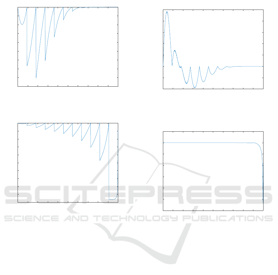
3.3.3 Evaluation using Lookup-tables
We pre-evaluate the polynomials at K = 10
7
evenly
spaced points, x
0
,..., x
K
between 0 and 1, using infi-
nite precision arithmetic and then truncate and store
the results. At runtime we evaluate W
j
(x) by find-
ing i such that x
i
is the closest value to x and return
W
j
(x) ≈ W
j
(x
i
). Here is a pseudo-code of the full pro-
cedure:
//j selects W_j
Lookuptable(x, j)
i=round(x*(K-1));
return W_j[i];
The tables are constructed in such a way that we
can use the same index to get the values of all of the
W
j
functions, and furthermore by weaving the tables
together we can evaluate all four of them by read-
Verification of a Numerical Solution to a Collocation Problem
591

0 0.1 0.2 0.3 0.4 0.5 0.6 0.7 0.8 0.9 1
-900
-800
-700
-600
-500
-400
-300
-200
-100
0
Figure 7: Absolute error as a function of x of W
4
using
Lookup-table. Note the scale on the y-axis is ×10
0
.
0 0.1 0.2 0.3 0.4 0.5 0.6 0.7 0.8 0.9 1
-1
-0.9
-0.8
-0.7
-0.6
-0.5
-0.4
-0.3
-0.2
-0.1
0
× 10
-5
Figure 8: Relative error as a function of x of W
4
using
Lookup-table. Note the scale on the y-axis is ×10
−5
.
ing twice from memory, or even once on AVX2 capa-
ble machines. This is a significant performance boost
compared to the Horner’s method, see table 1. As for
the absolute error see figure 7. This kind of sawtooth
shape is typical for Lookup-tables, however, note that
the absolute error is high for x close to 0 but stabilizes
when x gets closer 1. Since the true value of the func-
tion W
4
close to 0 is very high, this translates to a low
relative error around 0, see figure 8.
3.3.4 Lookup-tables with Linear Interpolation
One improvement on the Lookup-table method de-
scribed in the previous section is to use linear interpo-
lation between the lookup values to get more accurate
evaluations at the cost of some processing time. Here
is a pseudo-code for the procedure:
Lookuptable_interpolate(x,j)
i=floor(x*(K-1));
interpolant:=(x-x_n[i])/ ...
...(x_n[i+1]-x_n[i]);
return W_j[i] + ...
...interpolant*(W_j[i+1]-W_j[i]);
0 0.1 0.2 0.3 0.4 0.5 0.6 0.7 0.8 0.9 1
-4
-2
0
2
4
6
8
10
× 10
-5
Figure 9: Absolute error as a function of x of W
4
using
Lookup-table with interpolation. Note the scale on the y-
axis is ×10
−5
.
0 0.1 0.2 0.3 0.4 0.5 0.6 0.7 0.8 0.9 1
-12
-10
-8
-6
-4
-2
0
2
× 10
-10
Figure 10: Relative error as a function of x of W
4
using
Lookup-table with interpolation. Note the scale on the y-
axis is ×10
−10
.
There is a significant increase in accuracy, see fig-
ure 9, but this method requires more memory access
than the previous method.
3.3.5 Combination of Lookup-table Methods
As noted in the previous sections, the accuracy of the
Lookup-table method is quite good when x is close
to 1, therefore we propose the following method: we
start by selecting a cutoff value b between 0 and
1, then when we evaluate W
j
(x) we use the simple
lookup method if x ≥ b, otherwise we use the Lookup-
table with interpolation.
Lookuptable_combined(x,j)
if(x>=b)
return Lookuptable(x,j);
else
return Lookuptable_interpolate(x,j);
Note the large absolute error around the value
x = 0.8 in figure 11 translates to a low relative error of
CTDE 2018 - Special Session on Control Theory and Differential Equations
592

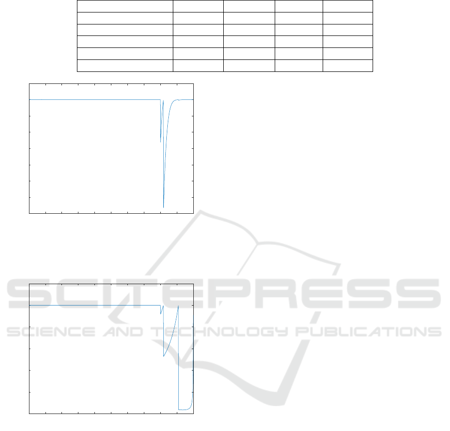
Table 1: Total execution time to evaluate the functions W
i
, i = 1,2,3,4, at 10
7
different points, using a single thread.
Method / Processor i5-8250U i5-3210M i5-2500k i7-4790K
Horner’s method 548.1ms 721ms 657.8ms 395ms
Simple Lookup-table 125.8ms 152.7ms 146.7ms 105ms
Lookup-table interp. 165.5ms 231.9ms 216.9ms 128ms
Lookup-table comb. 148.2ms 187.6ms 172.5ms 105ms
Hardcoded 171.5ms 214.8ms 199.8ms 107ms
0 0.1 0.2 0.3 0.4 0.5 0.6 0.7 0.8 0.9 1
-0.07
-0.06
-0.05
-0.04
-0.03
-0.02
-0.01
0
0.01
Figure 11: Absolute error as a function of x of W
4
using
Lookup-table with b = 0.8. Note the scale on the y-axis is
×10
0
.
0 0.1 0.2 0.3 0.4 0.5 0.6 0.7 0.8 0.9 1
-10
-8
-6
-4
-2
0
2
× 10
-6
Figure 12: Relative error as a function of x of W
4
using
Lookup-table with b = 0.8. Note the scale on the y-axis is
×10
−6
.
8 · 10
−6
, see figure 12. The value of b = 0.8 was em-
pirically determined to give the best tradeoff between
speed and accuracy.
4 CONCLUSIONS
We compared different methods to evaluate poly-
nomials stemming from Wendland’s compactly sup-
ported radial basis functions. In our application for
rigidly verifying the negativity of Lyapunov functions
computed for stochastic differential equations these
polynomials have to be evaluated at numerous points
and this has to be done with sufficient accuracy. Table
1 shows how long it takes to evaluate the polynomials
W
1
, W
2
, W
3
, and W
4
at 10
7
different points on different
processors. The fastest method is to use a Lookup-
table, but it is too inaccurate for practical use, at least
in our application. Using linear interpolation between
the lookup-values produced much more accurate re-
sults, but the method is considerably slower. A more
efficient method that is sufficiently accurate is to use
linear interpolation between the lookup-values in the
most troublesome areas of the Lookup-table, and just
use simple Lookup-table otherwise. Hardcoding the
polynomials in factorized form as in equations (7)-
(10) is both very fast, although not as fast as using
a Lookup-table, and very accurate. Horner’s method
should be avoided since it produces inaccurate results
and is slow. The inaccuracy is supposedly due to the
multiple zero at 1 of the functions W
i
.
ACKNOWLEDGEMENTS
The research for this paper was supported by the Ice-
landic Research Fund (Rann
´
ıs) in the project ‘Lya-
punov Methods and Stochastic Stability’ (152429-
051), which is gratefully acknowledged.
REFERENCES
Bjornsson, H., Gudmundsson, S., Giesl, P., Hafstein, S., and
Scalas, E. (2018). Computation of the stochastic basin
of attraction by rigorous construction of a Lyapunov
function. submitted.
Giesl, P. (2007). Construction of Global Lyapunov Func-
tions Using Radial Basis Functions, volume 1904
of Lecture Notes in Mathematics. Springer-Verlag,
Berlin.
Giesl, P. (2008). Construction of a local and global Lya-
punov function using Radial Basis Functions. IMA J.
Appl. Math., 73(5):782–802.
Giesl, P. and Wendland, H. (2007). Meshless collocation:
error estimates with application to dynamical systems.
SIAM J. Numer. Anal., 45(4):1723–1741.
Verification of a Numerical Solution to a Collocation Problem
593

Gr
¨
une, L. and Camilli, F. (2003). Characterizing attraction
probabilities via the stochastic Zubov equation. Dis-
crete Contin. Dyn. Syst. Ser. B, 3(3):457–468.
Gudmundsson, S. and Hafstein, S. (2018). Probabilistic
basin of attraction and its estimation using two Lya-
punov functions. Complexity, Article ID:2895658.
Hafstein, S., Gudmundsson, S., Giesl, P., and Scalas,
E. (2018). Lyapunov function computation for au-
tonomous linear stochastic differential equations us-
ing sum-of-squares programming. Discrete Contin.
Dyn. Syst. Ser. B, 2(23):939–956.
Mohammed, N. and Giesl, P. (accepted). Grid refinement in
the construction of Lyapunov functions using Radial
Basis Functions. Discrete Contin. Dyn. Syst. Ser. B.
Wendland, H. (1998). Error estimates for interpolation by
compactly supported Radial Basis Functions of mini-
mal degree. J. Approx. Theory, 93:258–272.
CTDE 2018 - Special Session on Control Theory and Differential Equations
594