Usability of Concordance Indices in FAST-GDM Problems

Marcelo Loor

1,2

, Ana Tapia-Rosero

and Guy De Tr

Dept. of Telecommunications and Information Processing, Ghent University,

Sint-Pietersnieuwstraat 41, B-9000, Ghent, Belgium

Dept. of Electrical and Computer Engineering, ESPOL Polytechnic University,

Campus Gustavo Galindo V., Km. 30.5 Via Perimetral, Guayaquil, Ecuador

Keywords:

Flexible Consensus Reaching, Group Decision-Making, Intuitionistic Fuzzy Sets, IFS Contrasting Charts.

Abstract:

A ﬂexible attribute-set group decision-making (FAST-GDM) problem boils down to ﬁnding the most suitable

option(s) with a general agreement among the participants in a decision-making process in which each option

can be described by a ﬂexible collection of attributes. The solution to such a problem can involve a consensus

reaching process (CRP) in which the participants iteratively try to reach a general agreement on the best

option(s) based on the attributes that are relevant for each participant. A challenging task in a CRP is the

selection of an adequate method to determine the level of concordance between the evaluations given by each

participant and the collective evaluations computed for the group. To gain insights in this regard, we performed

a pilot test in which a group of persons were asked to estimate the level of concordance between individual and

collective evaluations obtained while other participants tried to solve a FAST-GDM problem. The perceived

concordance levels were compared with several theoretical concordance indices based on similarity measures

designed to compare intuitionistic fuzzy sets. This paper presents our ﬁndings on how each of the chosen

theoretical concordance indices reﬂected the perceived concordance levels.

1 INTRODUCTION

Consider a situation in which a group of viniculturists

are trying to reach a consensus about the best grape-

vine(s) for winemaking from a collection of grapevi-

nes that have been developed for the industry. In this

situation, a consensus can be reached using a process

where the viniculturists, under the supervision of a

moderator, can iteratively reconsider their evaluations

to be in agreement with the group and, thus, to decide

on the best grapevine(s) for winemaking (Bouyssou

et al., 2013). Assuming that the viniculturists have a

similar expertise, the moderator can ask them to eva-

luate each grapevine (i.e., each option) using a prede-

ﬁned collection of attributes, which denote the featu-

res or characteristics inherent to any of the grapevi-

nes under evaluation. As such, this situation can be

deemed to be an example of a multi-attribute group

decision-making (MA-GDM) problem (Dong et al.,

2016; Liu et al., 2016).

A different situation is one in which a heteroge-

neous group of participants have different opinions

on how the attributes (or features) of the given op-

tions should be evaluated. In this case, the problem

of ﬁnding a consensus with a ﬂexible collection of

attributes comes to light. As an example, one can

consider another situation where three untrained vi-

niculturists, say Alice, Bob and Chloe, are trying to

reach a consensus on the best grapevine(s) for wine-

making from the aforementioned collection of grape-

vines: while Alice considers that one of the grape-

vines, say ‘GV1’, is almost the best for winemaking

due to its reddish color, Bob considers this grapevine

to be unacceptable for winemaking because it is ex-

pensive; meanwhile, Chloe considers that ‘GV1’ is a

good grapevine for winemaking because of its appe-

tizing aroma, but it is not the best due to its strong

ﬂavor. Notice in this example that, since they are un-

trained viniculturists, Alice, Bob and Chloe evaluate

‘GV1’ according to the attributes that each of them

might consider to be relevant on this grapevine for

deciding whether or not it is the best for winemaking.

In this case, a consensus can be reached using a pro-

cess where these persons iteratively reconsider their

evaluations based on the attributes of the grapevines

that were initially unobserved by some of them but

observed by others. This last situation can be seen as

an example of a ﬂexible attribute-set group decision-

making (FAST-GDM) problem (Loor et al., 2018).

The solution to such group decision-making pro-

Loor, M., Tapia-Rosero, A. and De Tré, G.

Usability of Concordance Indices in FAST-GDM Problems.

DOI: 10.5220/0006956500670078

In Proceedings of the 10th International Joint Conference on Computational Intelligence (IJCCI 2018), pages 67-78

ISBN: 978-989-758-327-8

blems can involve a consensus reaching process

(CRP) in which the participants (experts or non-

experts) iteratively try to reach a collective agreement

on the best option(s) (Kacprzyk and Fedrizzi, 1988;

Herrera et al., 1996; Kacprzyk and Zadro

zny, 2010).

A challenge in this process is to ﬁnd a consistently

good method by which one can determine the level of

concordance between the individual evaluations given

by a participant and the collective evaluations compu-

ted for the group.

To gain insights about what can be accepted as a

good indicator of the level of concordance in FAST-

GDM problems, we conducted a pilot test in which an

easy-to-reach group of persons were asked to make an

estimation of the level of concordance that they per-

ceive between the individual and the collective eva-

luations obtained during the iterations of a CRP in

a FAST-GDM problem. To make such estimations,

those persons were provided with IFS contrasting

charts, a novelty of this work, which depict the evalu-

ations characterized as intuitionistic fuzzy sets (IFSs)

(Atanassov, 1986; Atanassov, 2012). Then, those esti-

mations were compared with several theoretical con-

cordance indices to determine the usability of each

index. By means of such comparisons, we aim to de-

termine how well those theoretical concordance indi-

ces could reﬂect a perceived level of concordance in a

FAST-GDM problem.

It is worth mentioning that, although the CRP pro-

posed for FAST-GDM problems is based on an aug-

mented variant of IFSs called augmented Atanassov

intuitionistic fuzzy sets (Loor and De Tr

e, 2017a), in

this test we use similarity measures designed to com-

pare traditional IFSs because the computation of con-

cordance indices can be done by using only the mem-

bership and nonmembership levels (Loor et al., 2018).

A practical motivation in this regard is to study the ap-

plicability of the tools included in the IFS framework

to the solution of decision-making problems where

participants having different expertise are given the

freedom to perform positive or negative evaluations

according to what they consider to be relevant.

To present the results of the pilot test, this paper

has been structured as follows. In Section 2, we pre-

sent some preliminary concepts, as well as the formu-

lation of a FAST-GDM problem. Then, in Section 3,

we describe the pilot test and introduce the novel IFS

contrasting charts. Before concluding this paper, we

present the results and our ﬁndings in Section 4 and

some related work in Section 5.

2 PRELIMINARIES

When there are different opinions on how the attribu-

tes (or features) of a predeﬁned collection of potential

options should be evaluated, an evaluation might be

accompanied by some suggestions about what have

been focused on during the evaluation process. For

instance, in the second introductory example Alice

has considered that ‘GV1’ is almost the best grapevine

for winemaking due to its reddish color. To characte-

rize this kind of evaluations, the idea of an augmen-

ted appraisal degree (AAD) has been introduced in

(Loor and De Tr

e, 2017a). In the context of decision-

making, such an augmented appraisal degree idea can

be described as follows:

Consider a discrete collection X = {x

, ⋯, x

} of

potential solutions, called options, for a particular

problem, where each x

∈ X has a collection of fea-

tures F

. Consider also that a collection of suitable

options for this problem in X is denoted by A, i.e.,

A ⊆ X . Finally, consider a person P who has been as-

ked to evaluate the level to which an option x

∈ X sa-

tisﬁes the proposition “p : x

is a member of A.” With

these considerations, an augmented appraisal degree

of x

, say ˆµ

A@P

), is a pair µ

A@P

), F

)

that denotes the level µ

A@P

) to which x

satisﬁes

the proposition p, as well as the collection of features

) ∈ F

considered by P while appraising the

proposition p.

For instance, consider the collection of grapevines

X = {‘GV1’, ‘GV2’, ‘GV3’}. Consider also a unit in-

terval scale where 0 and 1 represent the lowest and

the highest level of satisﬁability respectively. In this

context, after denoting (the collection of) the best gra-

pevine(s) for winemaking by the letter A, one can

characterize Alice’s evaluation by ˆµ

A@Alice

(‘GV1’) =

0.9, {‘reddish color’}.

In the second introductory example, Chloe has

considered that ‘GV1’ is a good grapevine for wine-

making because of its appetizing aroma, but it is not

the best due to its strong ﬂavor. Notice is this case that

one can provide an evaluation denoting not only how

acceptable but also how unacceptable an option could

be. To characterize this kind of evaluations, the inclu-

sion of AADs into the deﬁnition of an IFS has been

proposed in (Loor and De Tr

e, 2017a). Such augmen-

ted version of an IFS, called augmented (Atanassov)

intuitionistic fuzzy set (AAIFS), can be described as

follows:

Keep X , A, p and P as given above. Recall

that x

∈ X has a collection of features F

and as-

sume that F = F

∪⋯ ∪F

. Assume also I = [0, 1].

Let ˆµ

A@P

)= µ

A@P

), F

) and

A@P

ν

A@P

), F

) in I, F be two AADs deno-

IJCCI 2018 - 10th International Joint Conference on Computational Intelligence

ting the evaluations given by P on how acceptable and

how unacceptable x

is for fulﬁlling the proposition p

respectively. In this context, an AAIFS is a collection

that describes the correspondence between each

∈ X and both ˆµ

A@P

) and

A@P

) through the

expression

={x

, ˆµ

A@P

)  (x

∈ X)

∧(0 ≤ µ

A@P

)+ν

A@P

) ≤ 1)}. (1)

Notice in this expression that the consistency condi-

tion, i.e., 0 ≤ µ

A@P

)+ν

A@P

) ≤ 1, has been inher-

ited from the original deﬁnition of an IFS (Atanassov,

1986; Atanassov, 2012). Hence, an AAIFS can be

used for the characterization of evaluations like the

given by Chloe even if the evaluations are marked by

hesitation. Because of this and given that an AAIFS

can be used in situations when no constraint on the

attributes of the collection of potential options has

been established, the AAIFS concept has been used

in the formulation of a FAST-GDM problem as fol-

lows (Loor et al., 2018):

Consider a discrete collection X = {x

, ⋯, x

} of

potential options for a particular problem, and con-

sider that A ⊆ X represents a collection of suitable

options for this problem. Consider also a collection

E = {E

, ⋯, E

} that represent a group of participants,

experts or non-experts, who were asked to evaluate to

which level each option in X is member of A. Let



x

, ˆµ

A@E

)  (x

∈ X)

∧



0 ≤ µ

A@E

)+ν

A@E

) ≤ 1



(2)

be an AAIFS characterizing the individual evaluati-

ons given by E

∈ E. Let

A ={x

, ˆµ

)  (x

∈ X)

∧(0 ≤ µ

)+ν

) ≤ 1)} (3)

be an AAIFS characterizing the collective evaluati-

ons computed for the group of participants E. Finally,

let cix(

A) be a function, called concordance in-

dex, that computes the level of concordance between

and

A, where a higher value denotes a higher

concordance between

and

A. In this context, a

FAST-GDM problem boils down to ﬁnding the most

suitable option(s) in such a way that the average of all

the concordance indices, i.e.,

∑

∈E

cix(

A),

is maximized.

As can be noticed, the computation of a concor-

dance index is a very inﬂuential step in a FAST-GDM

problem. For this reason, the selection of an adequate

method for its computation is deemed to be an impor-

tant and challenging task.

An option to perform such computation is through

a function, say S, that computes the similarity bet-

ween

and

A, i.e., a concordance index can be

computed by

cix(

A) = S(

A). (4)

As will be shown in the next section, in this work

we use similarity measures that have been designed

to compare traditional IFSs.

3 PILOT STUDY

As was mentioned in Section 1, the aim of this pa-

per is to study how well a theoretical concordance in-

dex could reﬂect a perceived level of concordance be-

tween individual and collective evaluations in FAST-

GDM problems. Hence in this section, we describe a

procedure to get evaluations from people with diffe-

rent opinions on how the attributes of the given opti-

ons should be evaluated. Then, we explain how this

procedure has been used to get evaluations from a he-

terogeneous group of participants who tried to reach

consensus about the best smooth dip(s) to pair with

banana chips. After that, we describe how the indivi-

dual and the collective evaluations given by the afore-

mentioned group of participants have been compared

by theoretical concordance indices and perceived le-

vels of concordance.

3.1 Getting Evaluations

To get evaluations from persons who express not only

the level to which but also the reasons why a potential

option is suitable (or unsuitable) for a problem, we

use a form like the one shown in Figure 1. Notice

that, through this kind of form, a person can indicate

how suitable and how unsuitable an option could be

along with (some of) the reasons that justify his/her

appraisal.

hardly

highly

suitable...

... due to

unsuitable...

To which degree option 1 is suitable for problem XYZ?

feature 01

feature 04

feature 03

Figure 1: Form for evaluating an option.

The evaluations of the potential options ﬁlled out

by a person, say P, in such a form can easily be cha-

racterized as an AAIFS by means of the following

procedure:

Usability of Concordance Indices in FAST-GDM Problems

Consider a discrete collection X = {x

, ⋯, x

} of

potential options for the problem under study, and

consider that A ⊆ X represents a collection of suit-

able options for this problem. Then, consider that

the levels of suitability and unsuitability ﬁlled out

by P for any x

∈ X can be linked to two values in

a unit interval scale, say ˇµ

A@P

) and

A@P

) re-

spectively, where 1 denotes the highest value and 0

the lowest. Finally, consider that the features ﬁl-

led out for any x

∈ X can be included in two col-

lections, say F

A@P

) and F

A@P

). With these

considerations, compute η = max(1, (ˇµ

A@P

) +

A@P

))), ∀x

∈ X . After that, obtain an AAIFS

element x

, ˆµ

A@P

) for each option x

∈

X such that ˆµ

A@P

) = ˇµ

A@P

)η, F

A@P

) and

A@P

) = 

A@P

)η, F

A@P

).

Round

...

evaluation

aggregation

Figure 2: Getting evaluations.

We followed the above procedure to obtain the

evaluations from 11 persons, 6 women and 5 men,

who tried to reach consensus about the best smooth

dip(s), among 3 potential dips, to pair with banana

chips. This CRP was modeled using the notation in-

troduced in Section 2 as follows: the collection of po-

tential dips was denoted by X = {x

, x

}; the col-

lection of the best smooth dip to pair with banana

chips was denoted by A; the group of participants was

denoted by E = {E

, ⋯, E

}; the individual evaluati-

ons given any participant E

∈ E were represented by

an AAIFS

; and the collective evaluations com-

puted for the group were represented by an AAIFS

A (see Figure 2). This means that 12 AAIFSs (1

AAIFS representing the collective evaluations and 11

AAIFSs representing the individual evaluations) were

obtained in each of the 2 rounds completed by these

11 persons. In the next part, we show how these eva-

luations have been compared to each other.

3.2 Contrasting Evaluations

To compare a collection of individual evaluations, say

, with the collection of collective evaluations,

say

A, obtained during each round of the CRP, we use

theoretical concordance indices and perceived level of

concordance as explained below.

3.2.1 Theoretical Concordance Indices

Round

quantication

of concordance (cix)

XVBr-0.5

SK1

SK2

SK3

SK4

cix ( , )

XVBr-0.5

cix ( , )

SK1

cix ( , )

SK2

cix ( , )

SK3

cix ( , )

SK4

Figure 3: Quantiﬁcation of theoretical concordance indices.

The concordance index between each

and

A was computed by means of (4), where S was cho-

sen among ﬁve (conﬁgurations of) similarity mea-

sures designed to compare traditional IFSs, namely

XVBr-0.5 (Loor and De Tr

e, 2017b), SK1, SK2, SK3

and SK4 (Szmidt and Kacprzyk, 2004) (see Figure 3).

A ﬂat operator, ê ⋅ ⊩, which turns an AAIFS into an

IFS by excluding the collections of features recorded

in each AAIFS element, was used for converting

and

A into two IFSs, say J and A respectively, that are

used as input for any of the chosen similarity measu-

res. Regarding XVBr-0.5, it refers to a conﬁguration

(J, A) = ∆

⋅S

(J, A), (5)

in which α has been set to 0.5. In this equation,

∆

∈ [0, 1] is a factor that was computed through

the method spotRatios proposed in (Loor and De Tr

2017b) and S

(J, A) is given by

(J, A) = 1 −



i=1



(µ

)−µ

)) (6)

+ α(h

)−h

))



With respect to SK1, SK2, SK3 and SK4, they refer to

following similarity measures:

SK1

(J, A) = 1 − f (l(J, A), l(J, A

)), (7)

SK2

(J, A) =

1 − f (l(J, A), l(J, A

))

1 + f (l(J, A), l(J, A

))

, (8)

SK3

(J, A) =

(1 − f (l(J, A), l(J, A

)))

(1 + f (l(J, A), l(J, A

)))

(9)

and

SK4

(J, A) =

− f (l(J,A),l(J,A

))

−e

−1

1 −e

−1

. (10)

IJCCI 2018 - 10th International Joint Conference on Computational Intelligence

Herein, A

is the complement of A, i.e.,

= {x

, ν

), µ

)(x

∈ X) (11)

∧(0 ≤ µ

)+ν

) ≤ 1)},

l(J, A) has been set as the Hamming distance between

J and A (Szmidt and Kacprzyk, 2004), i.e.,

l(J, A)=



i=1



µ

)−µ

)+ (12)

+ν

)−ν

)+h

)−h

)



and

f (l(J, A), l(J, A

)) =

l(J, A)

l(J, A)+l(J, A

)

. (13)

The interest reader is referred to (Loor and De Tr

2017c) for an open-source implementation of the

above-mentioned similarity measures.

To obtain the perceived levels of concordance bet-

ween each

and

A, the AAIFSs were graphically

represented by means of IFS contrasting charts as ex-

plained in the next part.

3.2.2 Perceived Levels of Concordance

Aiming to facilitate the interpretation of the evaluati-

ons given by a person or computed for a group during

a CRP, we propose a novel visual representation of an

IFS, which is called IFS contrasting chart or IFSCC

for short.

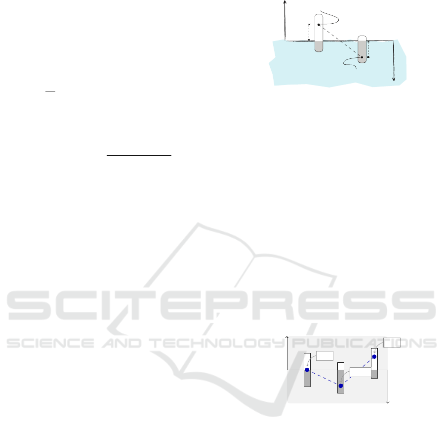
The idea behind an IFSCC can be described

through the following analogy. Consider that the eva-

luation of an option, say x

, is a buoy ﬂoating on the

surface of the sea. The air column inside this buoy

corresponds to the level to which x

is a suitable op-

tion, i.e., the air column corresponds to µ

). Like-

wise, the ballast in the buoy corresponds to the level

to which x

is an unsuitable option, i.e., the ballast

corresponds to ν

). This means that the buoyancy

of the buoy, say ρ

), results from the difference

between µ

) and ν

), i.e., the buoyancy corre-

sponds to ρ

) = µ

)−ν

). While a positive

value of ρ

) suggests that x

is a suitable option,

a negative value suggests that x

is an unsuitable op-

tion. The height of buoy is limited to the unit inter-

val [0, 1] because of the consistency condition, i.e.,

0 ≤ µ

)+ν

) ≤ 1, which is expressed in the de-

ﬁnition of an IFS. Figure 4 illustrates the evaluations

of two options, x

and x

, using this analogy.

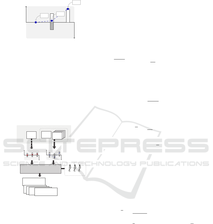
We can use the above analogy to represent the ap-

praisal levels in an AAIFS, say

, which charac-

terizes the evaluations of the collection of potential

dips performed by person E

during the ﬁrst round.

This representation is shown in Figure 5. Notice in

(x )

above sea level => suitable

below sea level => unsuitable

Figure 4: Idea behind an IFS contrasting chart.

this ﬁgure that the collection of potential dips is de-

noted by X = {x

, x

}. Notice also that the ‘buoy’

related to dip x

has equal parts of ‘air’ and ‘bal-

lasts’, i.e., µ

) = ν

), and, thus, the buoyancy

of x

is 0. This suggests that x

has some ‘positive’

features but also some ‘negative’ features that make

to think that x

neither satisﬁes nor dissatisﬁes

the membership in the collection of the best smooth

dips to pair with banana chips. In a similar way,

notice that the ‘buoy’ related to dip x

has less ‘air’

than ‘ballasts’ and, thus, x

has a negative buoyancy

(ρ

) = −0.48). This indicates that x

might not be

included by E

in the collection of the best smooth

dips. Finally, notice that the ‘buoy’ related to dip x

has more ‘air’ than ‘ballasts’ and, thus, x

has a posi-

tive buoyancy (ρ

) = 0.39). This suggests that E

might include x

in the collection of the best smooth

dips.

0 0

0.00

−0.48

0.39

Figure 5: Evaluations of the dips x

, x

and x

given by E

It is worth mentioning that, although the hesita-

tion margin, i.e., h

) = 1 −(µ

)+ν

)) (Ata-

nassov, 1986; Atanassov, 2012), is not explicitly de-

picted in an IFSCC, it can be inferred. For instance,

Figure 6 depicts the evaluations given by E

. Notice

that µ

) and ν

) are equal to 0. This suggests

that the evaluation of dip x

has been missed or that

did not try dip x

during the ﬁrst round. Hence,

considering x

as a member (or not) of the collection

of the best dips is marked by a high hesitation in this

case.

Notice in Figure 5 and Figure 6 that an IFSCC

shows a holistic view of the evaluations given by a

participant in a CRP. Thus, to obtain the perceived

level of concordance between the individual and col-

lective evaluations in the CRP about the best smooth

Usability of Concordance Indices in FAST-GDM Problems

0 0

0.00

0.10

0.83

Figure 6: Evaluations of the dips x

, x

and x

given by E

dips, we built the IFSCCs of the 24 AAIFSs (22 re-

presenting individual evaluations and 2 representing

collective evaluations) obtained after the 2 rounds of

this CRP.

We made use of those IFSCCs, which are depicted

in Figures 12 and 13 (see Appendix), to make 22 pairs

of IFSCCs in such a way that the individual evaluati-

ons given by each participant could be compared with

the computed collective evaluations in each round –

i.e., 11 pairs of IFSCCs corresponding to pairs of

AAIFSs 

A, j = 1, ⋯, 11, were built for each

round.

Round

... ...

@ E

quantication

of perceived concordance (PLoC)

PLoC( , )

Figure 7: Quantiﬁcation of perceived levels of concordance.

Using those 22 pairs of IFSCCs, we asked a group

of 13 persons having managerial roles to quantify the

level of concordance that each of them perceives bet-

ween each pair of IFSCCs (see Figure 7). To indicate

so, the use of a unit interval scale where 1 and 0 repre-

sent the highest and the lowest level of concordance

respectively was recommended.

3.2.3 Theoretical vs. Perceived Concordance

To compare the perceived levels of concordance gi-

ven by the group of 13 people with the theoretical

concordance indices computed by the similarity me-

asures mentioned in Section 3.1, we followed two

approaches: a macro approach in which the average

of the perceived levels of concordance is contrasted

with each concordance index; and a micro approach

in which each perceived level of concordance is con-

trasted with each concordance index. These compa-

risons are as follows. Consider that P = {P

, ⋯, P

}

represents the group of the 13 persons. Consider also

that PLoC

(

A) represents the level of concor-

dance between

and

A perceived by any P

∈ P.

With these considerations, in the macro comparison

we ﬁrst compute the average of the perceived levels

for each pair 

A by means of

PLoC(

A) =

P



∈P

(PLoC

(

A)), (14)

where P denotes the number of persons having ma-

nagerial roles. Then, we compute the absolute error

between the average of the perceived level of con-

cordance and a given concordance index, say cix, for

each pair 

A by means of

∆

cix

(

A) = PLoC(

A)−cix(

A),

(15)

where ⋅  denotes the absolute value. After that, we

compute a macro mean absolute error by means of

∆

cix

E



∈E

∆

cix

(

A), (16)

where E represents the number of participants in E.

In this case, a value of ∆

cix

close to 0 means that cix

reﬂects well the perceived level of concordance.

Regarding the micro comparison, we compute for

a given person in P, say P

, the absolute error bet-

ween the perceived level of concordance and a given

concordance index, say cix, for each pair 

A

by means of

cix,P

(

A)= PLoC

(

A)−cix(

A).

(17)

Then, we aggregate all these absolute errors through

a micro mean absolute error computed by

cix

E×P



∈E,P

∈P

cix,P

(

A). (18)

A value of δ

cix

close to 0, as analogous to ∆

cix

, means

that cix reﬂects well the perceived level of concor-

dance.

The results obtained after performing the afore-

mentioned comparisons are shown in the next section.

4 RESULTS AND DISCUSSION

In this section, we present the results and our ﬁndings

on how well each of the chosen theoretical concor-

dance indices reﬂected the perceived levels of con-

cordance.

IJCCI 2018 - 10th International Joint Conference on Computational Intelligence

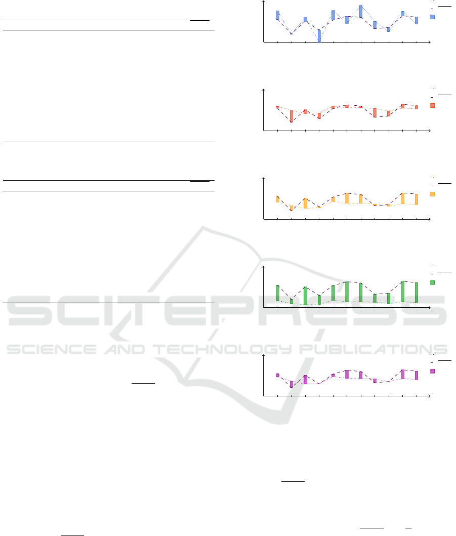
Table 1: Theoretical Concordance Indices and Average of

Perceived Levels of Concordance (Round 1).

Pair XVBr-0.5 SK1 SK2 SK3 SK4 PLoC



A 0.75 0.58 0.41 0.17 0.46 0.54



A 0.19 0.48 0.32 0.10 0.36 0.20



A 0.59 0.41 0.26 0.07 0.29 0.50



A 0.00 0.42 0.27 0.07 0.30 0.29



A 0.76 0.59 0.42 0.18 0.47 0.53



A 0.45 0.55 0.38 0.14 0.43 0.62



A 0.88 0.55 0.38 0.14 0.42 0.59



A 0.50 0.53 0.36 0.13 0.41 0.32



A 0.25 0.47 0.31 0.10 0.35 0.35



A 0.74 0.54 0.37 0.14 0.42 0.63



A 0.43 0.52 0.35 0.12 0.40 0.60

Table 2: Theoretical Concordance Indices and Average of

Perceived Levels of Concordance (Round 2).

Pair XVBr-0.5 SK1 SK2 SK3 SK4 PLoC



A 0.43 0.49 0.33 0.11 0.37 0.43



A 0.40 0.52 0.35 0.13 0.40 0.18



A 0.00 0.34 0.21 0.04 0.24 0.15



A 0.20 0.50 0.34 0.11 0.38 0.14



A 0.68 0.61 0.43 0.19 0.48 0.43



A 0.55 0.65 0.48 0.23 0.53 0.68



A 0.54 0.66 0.49 0.24 0.54 0.76



A 0.53 0.45 0.29 0.08 0.33 0.36



A 0.50 0.61 0.44 0.19 0.49 0.46



A 0.53 0.49 0.33 0.11 0.37 0.52



A 0.56 0.65 0.48 0.23 0.53 0.50

4.1 Results

The computed theoretical concordance indices, iden-

tiﬁed by XVBr-0.5, SK1, SK2, SK3 and SK4, along

with the macro average of the perceived levels of con-

cordance, which is denoted by PLoC and computed

by (14), are shown in Table 1 and Table 2: while the

data in the former table correspond to the 11 pairs of

IFSCCs obtained during the ﬁrst round (see Figure 12

in Appendix), the data in the latter table correspond

to the 11 pairs of IFSCCs obtained during the second

round (see Figure 13 in Appendix).

We make use of the data in the aforementioned ta-

bles as inputs of (15) to compute ∆

cix

(

A) for

each of the theoretical concordance indices. The re-

sults are depicted as bars in Figure 8 (Round 1) and

Figure 9 (Round 2). For instance, in Figure 8(a)

the lowest and the highest absolute errors between

XVBr-0.5 and PLoC are related to the pairs 

A

and 

A, which result from ∆

XVBr-0.5

(

A) =

0.19 − 0.20 = 0.01 and ∆

XVBr-0.5

(

A) = 0 −

0.29 = 0.29 respectively.

For the sake of a better macro comparison, a fre-

quency distribution of the absolute errors correspon-

ding to the two rounds are depicted in Figure 10.

As an example of the frequency distribution, in Fi-

Concordance Level

⟨

A⟩

⟨

A⟩

⟨

A⟩

⟨

A⟩

⟨

A⟩

⟨

A⟩

⟨

A⟩

⟨

A⟩

⟨

A⟩

⟨

A⟩

⟨

A⟩

XVBr-0.5

PLoC

Abs.Err.

(a) XVBr-0.5.

Concordance Level

⟨

A⟩

⟨

A⟩

⟨

A⟩

⟨

A⟩

⟨

A⟩

⟨

A⟩

⟨

A⟩

⟨

A⟩

⟨

A⟩

⟨

A⟩

⟨

A⟩

SK1

PLoC

Abs.Err.

(b) SK1.

Concordance Level

⟨

A⟩

⟨

A⟩

⟨

A⟩

⟨

A⟩

⟨

A⟩

⟨

A⟩

⟨

A⟩

⟨

A⟩

⟨

A⟩

⟨

A⟩

⟨

A⟩

SK2

PLoC

Abs.Err.

Concordance Level

⟨

A⟩

⟨

A⟩

⟨

A⟩

⟨

A⟩

⟨

A⟩

⟨

A⟩

⟨

A⟩

⟨

A⟩

⟨

A⟩

⟨

A⟩

⟨

A⟩

SK3

PLoC

Abs.Err.

(d) SK3.

Concordance Level

⟨

A⟩

⟨

A⟩

⟨

A⟩

⟨

A⟩

⟨

A⟩

⟨

A⟩

⟨

A⟩

⟨

A⟩

⟨

A⟩

⟨

A⟩

⟨

A⟩

SK4

PLoC

Abs.Err.

(e) SK4.

Figure 8: Absolute Errors (Round 1).

gure 10(b) it is shown that, while 12 out of 22 (i.e.,

54.54%) of the computed absolute errors between

SK1 and PLoC are placed in the interval [0, 0.1],

6 out of 22 (i.e., 27.27%) are located in the inter-

val (0.1, 0.2]. The values computed by (16) are also

shown in Figure 10. For instance, the macro mean ab-

solute error between SK1 and PLoC, i.e., ∆

SK1

= 0.13,

is indicated in the center of Figure 10(b).

Regarding the comparisons using a micro appro-

ach, a frequency distribution of the results compu-

ted by (17) and (18) are depicted in Figure 11. In

Figure 11(c), e.g., it is shown that, while 68 out of

286 (i.e., 23.77%) of the computed absolute errors

between SK1 and PLoC are located in the interval

[0, 0.1], 74 out of 286 (i.e., 25.87%) are placed in the

Usability of Concordance Indices in FAST-GDM Problems

Concordance Level

⟨

A⟩

⟨

A⟩

⟨

A⟩

⟨

A⟩

⟨

A⟩

⟨

A⟩

⟨

A⟩

⟨

A⟩

⟨

A⟩

⟨

A⟩

⟨

A⟩

XVBr-0.5

PLoC

Abs.Err.

(a) XVBr-0.5.

Concordance Level

⟨

A⟩

⟨

A⟩

⟨

A⟩

⟨

A⟩

⟨

A⟩

⟨

A⟩

⟨

A⟩

⟨

A⟩

⟨

A⟩

⟨

A⟩

⟨

A⟩

SK1

PLoC

Abs.Err.

(b) SK1.

Concordance Level

⟨

A⟩

⟨

A⟩

⟨

A⟩

⟨

A⟩

⟨

A⟩

⟨

A⟩

⟨

A⟩

⟨

A⟩

⟨

A⟩

⟨

A⟩

⟨

A⟩

SK2

PLoC

Abs.Err.

Concordance Level

⟨

A⟩

⟨

A⟩

⟨

A⟩

⟨

A⟩

⟨

A⟩

⟨

A⟩

⟨

A⟩

⟨

A⟩

⟨

A⟩

⟨

A⟩

⟨

A⟩

SK3

PLoC

Abs.Err.

(d) SK3.

Concordance Level

⟨

A⟩

⟨

A⟩

⟨

A⟩

⟨

A⟩

⟨

A⟩

⟨

A⟩

⟨

A⟩

⟨

A⟩

⟨

A⟩

⟨

A⟩

⟨

A⟩

SK4

PLoC

Abs.Err.

(e) SK4.

Figure 9: Absolute Errors (Round 2).

Table 3: Macro and micro mean absolute errors.

XVBr-0.5 SK1 SK2 SK3 SK4

∆

cix

0.14 0.13 0.13 0.31 0.12

cix

0.21 0.21 0.22 0.33 0.21

interval (0.1, 0.2]. In this case, the micro mean abso-

lute error between SK2 and PLoC, i.e., δ

SK2

= 0.22, is

indicated in the center of Figure 11(c). The results are

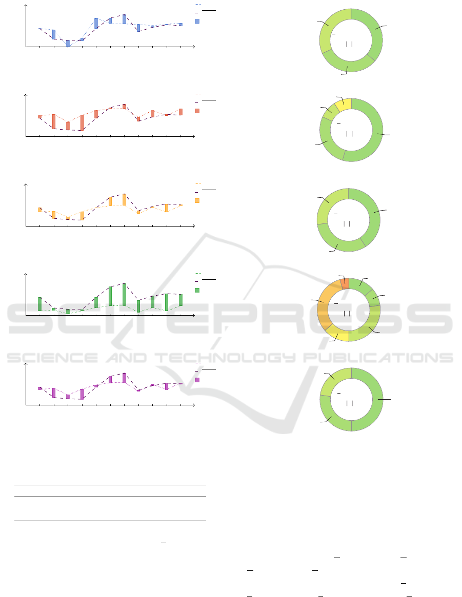
summarized in Table 3.

4.2 Discussion

The results listed in Table 3 suggest that the con-

cordance indices (based on the similarity measures)

∆

XVBr-0.5

= 0.14

2 ×

E = 22

“[0, 0.1]”: 8 (36.36%)

“(0.1, 0.2]”: 7 (31.82%)

“(0.2, 0.3] ”: 7 (31.82%)

(a) XVBr-0.5.

∆

SK1

= 0.13

2 ×

E = 22

“[0, 0.1]”: 12 (54.54%)

“(0.1, 0.2]”: 6 (27.27%)

“(0.2, 0.3]”: 2 (9.09%)

“(0.3, 0.4]”: 2 (9.09%)

(b) SK1.

∆

SK2

= 0.13

2 ×

E = 22

“[0, 0.1]”: 9 (40.91%)

“(0.1, 0.2]”: 7 (31.82%)

“(0.2, 0.3] ”: 6 (27.27%)

∆

SK3

= 0.31

2 ×

E = 22

“[0, 0.1]”: 3 (13.64%)

“(0.1, 0.2]”: 2 (9.09%)

“(0.2, 0.3]”: 6 (27.27%)

“(0.3, 0.4]”: 3 (13.64%)

“(0.4, 0.5]”: 7 (31.82%)

“(0.5, 0.6] ”: 1 (4.54%)

(d) SK3.

∆

SK4

= 0.12

2 ×

E = 22

“[0, 0.1]”: 11 (50%)

“(0.1, 0.2]”: 6 (27.27%)

“(0.2, 0.3]”: 5 (22.73%)

(e) SK4.

Figure 10: Distribution of Abs. Errors (Macro compari-

sons).

XVBr-0.5, SK1, SK2 and SK4 reﬂect to an acceptable

extent the perceived level of concordance between the

individual and the collective evaluations.

As far as one can see, SK4 slightly outperforms

XVBr-0.5, SK1 and SK2 according to both the ma-

cro and the micro mean absolute errors. Notice that,

while the expression (∆

SK4

= 0.12) < (∆

SK1

= 0.13) ≤

(∆

SK2

=0.13) <(∆

XVBr-0.5

=0.14) holds for the macro

mean absolute errors, the expression (δ

SK4

= 0.21) ≤

(δ

SK1

= 0.21) ≤ (δ

XVBr-0.5

= 0.21) < (δ

SK2

= 0.22)

holds for the micro mean absolute errors. However,

such a slightly advantage of SK4 can disappear if so-

meone focuses only on the frequency of the abso-

IJCCI 2018 - 10th International Joint Conference on Computational Intelligence

XVBr-0.5

= 0.21

2 ×

E P = 286

“[0, 0.1]”: 97 (33.92%)

“(0.1, 0.2]”: 62 (21.68%)

“(0.2, 0.3]”: 54 (18.88%)

“(0.3, 0.4]”: 42 (14.69%)

“(0.4, 0.5]”: 15 (5

24%)

“(0.5, 0.6]”: 10 (3

.5%)

“(0.6, 0.7]”: 5 (1

75%)

“(0.7, 0.8]”: 1 (0

35%)

(a) XVBr-0.5.

SK1

= 0.21

2 ×

E P = 286

“[0, 0.1]”: 76 (26.57%)

“(0.1, 0.2]”: 65 (22.73%)

“(0.2, 0.3]”: 57 (19.93%)

“(0.3, 0.4]”: 56 (19.58%)

“(0.4, 0.5]”: 25 (8

74%)

“(0.5, 0.6]”: 7 (2.45%)

(b) SK1.

SK2

= 0.22

2 ×

E P = 286

“[0, 0.1]”: 68 (23.77%)

“(0.1, 0.2]”: 74 (25.87%)

“(0.2, 0.3]”: 70 (24.48%)

“(0.3, 0.4]”: 40 (13.98%)

“(0.4, 0.5]”: 19 (6

64%)

“(0.5, 0.6]”: 12 (4.19%)

“(0.6, 0.7]”: 3 (1

05%)

SK3

= 0.33

2 ×

E P = 286

“[0, 0.1]”: 64 (22.38%)

“(0.1, 0.2]”: 41 (14.34%)

“(0.2, 0.3]”: 31 (10.84%)

“(0.3, 0.4]”: 31 (10.84%)

“(0.4, 0.5]”: 42 (14.69%)

“(0.5, 0.6]”: 34 (11.89%)

“(0.6, 0.7]”: 24 (8.39%)

“(0.7, 0.8]”: 11 (3.85%)

“(0.8, 0.9]”: 8 (2

.8%)

(d) SK3.

SK4

= 0.21

2 ×

E P = 286

“[0, 0.1]”: 66 (23.08%)

“(0.1, 0.2]”: 71 (24.82%)

“(0.2, 0.3]”: 80 (27.97%)

“(0.3, 0.4]”: 41 (14.34%)

“(0.4, 0.5]”: 19 (6.64%)

“(0.5, 0.6]”: 8 (2 .8%)

“(0.6, 0.7]”: 1 (0

35%)

(e) SK4.

Figure 11: Distribution of Abs. Errors (Micro Compari-

sons).

lute errors between the concordance indices and the

average of perceived levels of concordance located in

the interval [0, 0.1] (i.e., ∆

cix

∈ [0, 0.1]) – notice in Fi-

gure 10 that the frequency of ∆

SK1

∈[0, 0.1], i.e., 12, is

slightly greater than the frequency of ∆

SK4

∈ [0, 0.1],

i.e., 11. That advantage can also disappear when so-

meone only takes into account the frequency of the

absolute errors between the concordance indices and

the perceived levels of concordance located in the in-

terval [0, 0.1] (i.e., δ

cix

∈[0, 0.1]) – notice in Figure 11

that the frequency of δ

XVBr-0.5

∈ [0, 0.1], i.e., 97, is

greater than the frequency of δ

SK4

∈ [0, 0.1], i.e., 66.

Hence, we can say that, although SK4 has a slightly

advantage, in this pilot study the concordance indi-

ces based on the similarity measures XVBr-0.5, SK1,

SK2 and SK4 are comparatively alike when reﬂecting

the perceived levels of concordance between the in-

dividual and the collective evaluations. A practical

implication of these results is that these concordance

indices can be accepted as good indicators of the level

of concordance in FAST-GDM problems.

Regarding the concordance index based on the si-

milarity measure SK3, the computed macro and mi-

cro mean absolute errors suggest that this index might

not reﬂect well the perceived level of concordance.

Notice in Figure 10(d) and Figure 11(d) that roughly

50% of the computed absolute errors are located in

the interval (0.30, 1].

It is worth mentioning that, although in the ﬁrst

round the individual evaluations characterized by

(see Figure 12(e)) and the collective evaluations

characterized by

A (see Figure 12(a)) can lead to po-

tential opposite decisions about the options x

, x

and

, the average of the perceived level of concordance

related to the pair 

A, i.e., PLoC(

A) =

0.29, is appreciably greater than the expected theo-

retical value for this case, i.e., 0 (Loor and De Tr

2017b). A potential explanation for this result might

be that a more clear indication of the potential deci-

sion that can be taken after studying the evaluations

represented in an IFSCC is needed. In this regard,

conducting a follow-up study in which the perceived

levels of concordance would be obtained by compa-

ring IFSCCs that have been augmented with additio-

nal information (e.g., an explicit ranking of the opti-

ons, or a linguistic summary about a potential deci-

sion (Kacprzyk and Zadro

zny, 2005)) is suggested.

Another suggested study concerns the use of sca-

les of measurement formed from linguistic labels such

as ‘highly concordant’ or ‘hardly concordant’ to map

or express the results of the concordance indices, as

well as the perceived levels of concordance (Her-

rera et al., 1996; Herrera et al., 1997). Since the

macro averages computed for the concordance indi-

ces XVBr-0.5, SK1, SK2 and SK4 are roughly 0.12,

we foresee that a scale consisting of 5 linguistic la-

bels, for instance ‘hardly concordant’, ‘not specially

concordant’,‘slightly concordant’,‘fairly concordant’

and ‘highly concordant’, can further improve the level

to which those concordance indices reﬂect the percei-

Usability of Concordance Indices in FAST-GDM Problems

ved levels of concordance.

5 RELATED WORK

Methods that obtain the level of concordance (or

agreement) between the evaluations given by two in-

dividuals by means of a similarity (or distance) me-

asure deﬁned in the IFS framework can be found in

the literature. For instance, in (Szmidt and Kacprzyk,

2002; Szmidt and Kacprzyk, 2003; Szmidt and Ka-

cprzyk, 2004) Szmidt and Kacprzyk proposed the use

of either similarity or distance measures between two

IFSs to compute the level of agreement between two

participants whose evaluations have been characteri-

zed as IFSs. However, to the best of our knowledge,

no empirical study oriented to determine how well the

results computed by such similarity measures reﬂect

the perceived levels of concordance in a consensus re-

aching process has been published so far.

Regarding the visual representations of IFSs, se-

veral geometrical interpretations of IFSs are availa-

ble in the literature. The standard interpretation, in

which the membership and the nonmembership com-

ponents, i.e., µ

(x) and ν

(x), are depicted in a com-

mon region (or band) of height 1, is the most accep-

ted visual representation of IFSs according to Atanas-

sov (Atanassov, 2012). A variant of the standard in-

terpretation is one in which is depicted (1 − ν

(x))

instead of ν

(x). This variant leads to a represen-

tation where each element in an IFS is depicted a

unit segment. Another representation, called IFS-

interpretational triangle, is based on a right triangle

having two sides of length 1: one for µ

(x) and the

other for ν

(x) (Atanassov, 1986; Atanassov, 2012).

While an advantage of the IFS-interpretational tri-

angle is that an operation over an IFS element can, in

general, be easily visualized, a disadvantage of this

representation is that a holistic view of all the IFS

elements can be unclear. As a variant of the IFS-

interpretational triangle, the idea of a ‘unit cube’ to

additionally represent the hesitation margin has been

introduced in (Szmidt and Kacprzyk, 2004). Using

a different approach, the representation of an IFS by

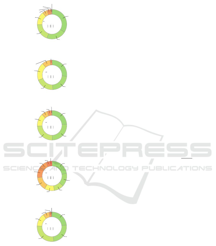
means of radar charts has been proposed in (Atanas-

sova, 2010). Since radar charts are typically used in

a business-oriented environment, an IFS radar chart

can be considered as a business-oriented representa-

tion of an IFS. However, the representation of the two

components in the same circle (or band) can be con-

fusing when the representation of the buoyancy of the

elements of an IFS is needed. Because of this, we

propose a novel business-oriented representation of

an IFS by means of an IFSCC. As could be noticed

throughout this paper, two bands, one for µ

(x) and

the other for ν

(x), are used within an IFSCC to de-

pict in a holistic way the buoyancy of each element in

an IFS.

6 CONCLUSIONS

In this paper, we have described a pilot study in which

several theoretical concordance indices based on si-

milarity measures designed to compare intuitionis-

tic fuzzy sets (IFSs) have been tested to determine

their usability in ﬂexible attribute-set group decision-

making (FAST-GDM) problems.

During the study, the evaluations obtained from

a group of participants who tried to ﬁnd a solution

for a FAST-GDM problem were characterized as aug-

mented Atanassov intuitionistic fuzzy sets (AAIFSs).

Then, each of those AAIFSs was graphically repre-

sented by means of a novel business-oriented repre-

sentation called IFS contrasting chart (IFSCC). After

that, a group of persons having managerial roles were

asked to estimate the level of concordance between

the individual and the collective evaluations depicted

respectively in two IFSCCs. The perceived levels of

concordance given by this group were then compared

to the values computed by the theoretical concordance

indices.

The results of this pilot study suggest that, among

the ﬁve theoretical concordance indices chosen for the

test, four reﬂected to an acceptable extent the percei-

ved level of concordance between the individual and

the collective evaluations. However, a more exten-

ded study should corroborate the usability of these

concordance indices in practical situations involving

FAST-GDM problems.

It was found a case in which the perceived level

of concordance between the individual and collective

evaluations is not the lowest even though such evalua-

tions lead to complete opposite decisions. A possible

explanation for this case might be that a more clear

indication of the potential decisions is needed in the

two IFSCCs representing such evaluations. Hence,

a follow-up study in which additional information

about a potential decision is incorporated into an IF-

SCC is suggested. Another suggested study concerns

the usability of scales of measurement formed from

linguistic labels to quantify both theoretical and per-

ceived concordance levels.

IJCCI 2018 - 10th International Joint Conference on Computational Intelligence

REFERENCES

Atanassov, K. T. (1986). Intuitionistic fuzzy sets. Fuzzy sets

and Systems, 20(1):87–96.

Atanassov, K. T. (2012). On Intuitionistic Fuzzy Sets The-

ory, volume 283 of Studies in Fuzziness and Soft Com-

puting. Springer Berlin Heidelberg, Berlin, Heidel-

berg.

Atanassova, V. (2010). Representation of fuzzy and intuiti-

onistic fuzzy data by radar charts. Notes on Intuitio-

nistic Fuzzy Sets, 16(1):21–26.

Bouyssou, D., Dubois, D., Prade, H., and Pirlot, M. (2013).

Decision Making Process: Concepts and Methods.

John Wiley & Sons.

Dong, Y., Xiao, J., Zhang, H., and Wang, T. (2016). Ma-

naging consensus and weights in iterative multiple-

attribute group decision making. Applied Soft Com-

puting, 48:80 – 90.

Herrera, F., Herrera-Viedma, E., and Verdegay, J. L. (1996).

A model of consensus in group decision making un-

der linguistic assessments. Fuzzy Sets and Systems,

78(1):73 – 87.

Herrera, F., Herrera-Viedma, E., and Verdegay, J. L. (1997).

A rational consensus model in group decision making

using linguistic assessments. Fuzzy Sets and Systems,

88(1):31 – 49.

Kacprzyk, J. and Fedrizzi, M. (1988). A ‘soft’ measure of

consensus in the setting of partial (fuzzy) preferences.

European Journal of Operational Research, 34(3):316

– 325.

Kacprzyk, J. and Zadro

zny, S. (2005). Linguistic database

summaries and their protoforms: towards natural lan-

guage based knowledge discovery tools. Information

Sciences, 173(4):281 – 304. Dealing with Uncertainty

in Data Mining and Information Extraction.

Kacprzyk, J. and Zadro

zny, S. (2010). Soft computing and

web intelligence for supporting consensus reaching.

Soft Computing, 14(8):833–846.

Liu, Y., Fan, Z.-P., and Zhang, X. (2016). A method

for large group decision-making based on evaluation

information provided by participators from multiple

groups. Information Fusion, 29:132–141.

Loor, M. and De Tr

e, G. (2017a). On the Need for Augmen-

ted Appraisal Degrees to Handle Experience-Based

Evaluations. Applied Soft Computing, 54C:284 – 295.

Loor, M. and De Tr

e, G. (2017b). In a Quest for Suitable

Similarity Measures to Compare Experience-Based

Evaluations. In Merelo, J. J., Rosa, A., Cadenas, J. M.,

Correia, A. D., Madani, K., Ruano, A., and Filipe,

J., editors, Computational Intelligence: International

Joint Conference, IJCCI 2015 Lisbon, Portugal, No-

vember 12-14, 2015, Revised Selected Papers, volume

669 of Studies in Computational Intelligence, pages

291–314. Springer International Publishing.

Loor, M. and De Tr

e, G. (2017c). An open-source software

package to assess similarity measures that compare

intuitionistic fuzzy sets. In 2017 IEEE International

Conference on Fuzzy Systems (FUZZ-IEEE), pages 1–

Loor, M., Tapia-Rosero, A., and De Tr

e, G. (2018). Refo-

cusing attention on unobserved attributes to reach con-

sensus in decision making problems involving a hete-

rogeneous group of experts. In Kacprzyk, J., Szmidt,

E., Zadro

zny, S., Atanassov, K. T., and Krawczak,

M., editors, Advances in Fuzzy Logic and Technology

2017, pages 405–416, Springer International Publis-

hing.

Szmidt, E. and Kacprzyk, J. (2002). Evaluation of

agreement in a group of experts via distances bet-

ween intuitionistic fuzzy preferences. In Proceedings

First International IEEE Symposium Intelligent Sys-

tems, volume 1, pages 166–170 vol.1.

Szmidt, E. and Kacprzyk, J. (2003). A consensus rea-

ching process under intuitionistic fuzzy preference re-

lations. International Journal of Intelligent Systems,

18(7):837–852.

Szmidt, E. and Kacprzyk, J. (2004). A concept of simila-

rity for intuitionistic fuzzy sets and its use in group

decision making. In IEEE International Conference

on Fuzzy Systems, pages 1129–1134.

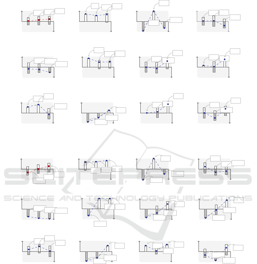
APPENDIX

Evaluations about the ‘best smooth dip’

This appendix presents the evaluations given by 11

persons who tried to reach a consensus about the best

smooth dip(s), among 3 potential dips, to pair with

banana chips. These evaluations have been graphi-

cally represented by means of IFS contrasting charts

(IFSCCs) (see Section 3.2).

Figure 12 shows the IFSCCs corresponding to the

evaluations given or computed during the ﬁrst round

of the consensus reaching process: while Figure 12(a)

represents the collective evaluations computed for the

group, Figures 12(b)-12(l) represent the individual

evaluations given by these 11 persons respectively.

In a similar way, Figure 13 shows the IFSCCs corre-

sponding to the evaluations given or computed during

the second round.

Usability of Concordance Indices in FAST-GDM Problems

0 0

0.04

0.13

0.21

(a)

0 0

0.7

0.55

0.65

(b)

0 0

−0.9

0.97

−0.63

(c)

0 0

0.04

0.06

−0.4

(d)

0 0

−0.16

−0.22

−0.49

(e)

0 0

0.83

0.47

0.50

(f)

0 0

0.00

−0.13

0.57

(g)

0 0

0.16

0.05

0.74

(h)

0 0

0.57

0.79

−0.14

(i)

0 0

−0.85

−0.45

0.25

(j)

0 0

0.00

0.10

0.83

(k)

0 0

0.00

−0.48

0.39

(l)

Figure 12: Evaluations obtained during Round 1.

0 0

−0.32

0.02

0.28

(a)

0 0

0.65

0.70

0.80

(b)

0 0

−1.00

1.00

−0.45

(c)

0 0

0.24

−0.29

−0.19

(d)

0 0

−0.70

−0.85

−0.90

(e)

0 0

−0.65

0.95 0.95

(f)

0 0

−0.78

−0.36

0.48

(g)

0 0

−0.82

−0.08

0.85

(h)

0 0

0.19

0.48

0.04

(i)

0 0

−0.90

−0.60

0.55

(j)

0 0

0.55

0.05

0.65

(k)

0 0

−0.33

−0.84

0.35

(l)

Figure 13: Evaluations obtained during Round 2.

IJCCI 2018 - 10th International Joint Conference on Computational Intelligence