An Investigation of Parameter Tuning in the Random Adaptive

Grouping Algorithm for LSGO Problems

Evgenii Sopov and Alexey Vakhnin

Department of System Analysis and Operations Research,

Reshetnev Siberian State University of Science and Technology,

Krasnoyarsk, Russia

Keywords: Large-Scale Global Optimization, Problem Decomposition, Variable Grouping, Cooperative Coevolution,

Evolutionary Algorithms.

Abstract: Large-scale global optimization (LSGO) is known as one of the most challenging problem for many search

algorithms. Many well-known real-world LSGO problems are not separable and are complex for

comprehensive analysis, thus they are viewed as the black-box optimization problems. The most advanced

algorithms for LSGO are based on cooperative coevolution with problem decomposition using grouping

methods. The random adaptive grouping algorithm (RAG) combines the ideas of random dynamic grouping

and learning dynamic grouping. In our previous studies, we have demonstrated that cooperative coevolution

(CC) of the Self-adaptive Differential Evolution (DE) with Neighborhood Search (SaNSDE) with RAG

(DECC-RAG) outperforms some state-of-the-art LSGO algorithms on the LSGO benchmarks proposed

within the IEEE CEC 2010 and 2013. Nevertheless, the performance of the RAG algorithm can be

improved by tuning the number of subcomponents. Moreover, there is a hypothesis that the number of

subcomponents should vary during the run. In this study, we have performed an experimental analysis of

parameter tuning in the RAG. The results show that the algorithm performs better when using

subcomponents of larger size. In addition, some improvement can be done by applying dynamic group

sizing.

1 INTRODUCTION

Optimization problems with many hundreds or

thousands of objective variables are called large-

scale global optimization (LSGO) problems. LSGO

is known as one of the most challenging problem for

many search techniques from the field of

mathematical programming and evolutionary

optimization. Many well-known real-world LSGO

problems are not separable and are complex for

comprehensive analysis, thus they are viewed as the

black-box optimization problems even the objective

function has analytical representation (using

mathematical formula).

Evolutionary algorithms (EAs) have proved their

efficiency at solving many complex real-world

black-box optimization problems. However, their

performance usually decreases when the

dimensionality of the search space increases. The

most advanced algorithms for LSGO are based on

cooperative coevolution (CC) with problem

decomposition using different grouping methods,

which decomposes LSGO problems into multiple

low-dimensional non-overlapping subcomponents.

Unfortunately, the nonseparability of real-world

LSGO problems excludes a straightforward variable-

based decomposition. There exist at least three types

of subcomponent grouping methods, including:

static, random dynamic and learning dynamic

grouping. The static grouping performs well only for

well-studied LSGO problems with regular

structures. The majority of state-of-the-art LSGO

techniques are based on the random grouping and

the learning-based grouping. The standard random

grouping can be applied to the wide range of

separable and non-separable LSGO problems, but it

does not use any feedback from the search process

for creating more efficient variables combinations.

Many learning dynamic grouping techniques

demonstrates too greedy adaptation, thus performs

well only with separable LSGO problems.

Sopov, E. and Vakhnin, A.

An Investigation of Parameter Tuning in the Random Adaptive Grouping Algorithm for LSGO Problems.

DOI: 10.5220/0006959802550263

In Proceedings of the 10th International Joint Conference on Computational Intelligence (IJCCI 2018), pages 255-263

ISBN: 978-989-758-327-8

255

In our previous study, we have proposed a novel

grouping technique that combines the ideas of the

random dynamic grouping and the learning dynamic

grouping. The approach is called the random

adaptive grouping (RAG). In our implementations,

the RAG is combined with cooperative coevolution

(CC) of the Self-adaptive Differential Evolution

(DE) with Neighborhood Search (SaNSDE) (the

whole search algorithm is called DECC-RAG). The

RAG starts with random subcomponents of an equal

predefined size. After some generations of the

DECC (so-called adaptation period), we estimate the

performance of each subcomponent. A portion of the

best subcomponents is saved for the next adaptation

period and for the rest of subcomponents we apply

the random grouping again. Such a feedback forms

different groups of variables and adaptively changes

them during the search.

In this study, we have performed an experimental

analysis of parameter tuning in the RAG. We have

estimated how the performance of the DECC-RAG

depends on the number of subcomponents. And, we

have implemented and investigated a modification

of the RAG with changing number of

subcomponents. In this paper, we will present the

experimental results for the LSGO CEC’10

benchmark only, because of great amount of time-

and resource-costly fitness evaluations.

Nevertheless, we will present and discuss the results

for the LSGO CEC’13 benchmark in our further

works and our presentation of the study.

The rest of the paper is organized as follows.

Section 2 describes related work. Section 3 describes

the proposed approach and experimental setups. In

Section 4 the results of numerical experiments are

discussed. In the Conclusion the results and further

research are discussed.

2 RELATED WORK

There exist a great variety of different LSGO

techniques that can be combined in two main

groups: non-decomposition methods and cooperative

coevolution (CC) algorithms. The first group of

methods are mostly based on improving standard

evolutionary and genetic operations. But the best

results and the majority of approaches are presented

by the second group. The CC methods decompose

LSGO problems into low dimensional sub-problems

by grouping the problem subcomponents. There are

many subcomponent grouping methods, including:

static grouping (Potter and Jong, 2000), random

dynamic grouping (Yang et al., 2008c) and learning

dynamic grouping (Omidvar et al., 2014, Liu and

Tang, 2013).

The first attempt to divide solution vectors into

several subcomponents using the static grouping was

proposed by (Potter and Jong, 1994). The approach

proposed by Potter and Jong decomposes a n-

dimensional optimization problem into n one-

dimensional problems (one subcomponent for each

variable). The CCGA employs CC framework and

the standard genetic algorithm (GA). Potter and Jong

had investigated two different modification of the

CCGA: CCGA-1 and CCGA-2. The CCGA-1

evolves each variable of objective in a round-robin

fashion using the current best values from the other

variables of function. The CCGA-2 algorithm

employs the method of random collaboration for

calculating the fitness of an individual by integrating

it with the randomly chosen members of other

subcomponents. Potter and Jong had shown that

CCGA-1 and CCGA-2 outperforms the standard

GA. Unfortunately, search techniques based on the

static grouping are inefficient for many non-

separable LSGO problems.

One of the most popular and well-studied random

grouping method had been proposed by Yang et al.

(Yang et al., 2007, Yang et al., 2008c) and uses a

DE-based CC method. The approach is called

DECC-G and it is used as a core conception for

many advanced techniques.

The learning dynamic grouping seems to be the

most perspective approach as it collects and uses

feedback information for improving the

decomposition stage. There were proposed a CC

algorithm based on the correlation matrix (Ray and

Yao, 2009), a CC with Variable Interaction Learning

(CCVIL) (Chen et al, 2010), an automated

decomposition approach (DECC-DG) with

differential grouping (Omidvar et al., 2014) and

many others. In our previous studies, we have

proposed the adaptive variable-size random

grouping algorithm (AVS-RG CC) based on the

Population-Level Dynamic Probabilities adaptation

model (Sopov, E., 2018). A good survey on LSGO

and methods is proposed in (Mahdavi et al., 2015).

The DECC-RAG algorithm (Vakhnin and

Sopov, 2018), which is investigated in this study,

combines the RAG approach with CC of the

SaNSDE. The SaNSDE algorithm have been

proposed by (Yang et al, 2008b). We have chosen

this algorithm because of its self-adaptive tuning of

parameters during optimization process. After each

regrouping of variable in the CC stage of the DECC-

RAG, we will deal with new optimization problems,

thus we need to choose a new efficient search

IJCCI 2018 - 10th International Joint Conference on Computational Intelligence

256

algorithm for each subcomponent. The SaNSDE

forms an efficient combination of DE’s parameters

(such as the type of mutation, the differential weight

and the crossover probability) in an automated (self-

adaptive) way.

The DECC-RAG operates with subcomponents

of equal size. This limitation excludes such

problems of the grouping methods as uneven

distribution of computational resources between

search algorithms and tuning the minimum and

maximum number of variables in groups. The RAG

divides the n-dimensional solution vector into m s-

dimensional sub-components (m x s = n), thus the

number of subcomponents is a parameter of the

algorithm. In our previous study we have estimated

the performance of the DECC-RAG with m = 10 on

the CEC’10 and CEC’13 LSGO benchmarks. The

experiments have shown that the proposed approach

outperforms on average some state-of-the-art

algorithms such as DMS-L-PSO dynamic multi-

swarm and local search based on PSO algorithm)

(Liang and Suganthan, 2005), DECC-G (cooperative

coevolution with random dynamic grouping based

on differential evolution) (Yang et al, 2008c),

MLCC (Multilevel cooperative coevolution based on

differential evolution) (Yang et al, 2008a) and

DECC-DG DECC-DG (cooperative coevolution

with differential grouping based on differential

evolution) (Omidvar et al, 2014).

It should be noted that the comprehensive

experimental analysis of LSGO algorithms is a

challenging problem because computations are time-

and resource-costly. According to the CEC LSGO

competition rules, the performance of a LSGO

algorithm is evaluated through 25 independent runs

on each benchmark problem using 3x106 fitness

evaluations in each independent run of the algorithm

(Li et al., 2013). In a case of serial computations

using 1 processor, the time for estimating the

performance of one algorithm (or one configuration

of an algorithm) is about 28 hours for LSGO

CEC’10 benchmark and is about 255 hours for

LSGO CEC’13 benchmark. We have implemented

all our numerical experiments using the C++

OpenMP framework for parallel computing. The

time of computations using 16 processors is about 5

hours for LSGO CEC’10 benchmark and is about 22

hours for LSGO CEC’13 benchmark.

3 EXPERIMENTAL SETUPS

The general scheme of the DECC-RAG can be

described by the following pseudo code:

Pseudocode of the DECC-RAG algorithm.

1: Set FEV_max, FEV_global, T,

FEV_local = 0;

2: An n-dimensional object vector is

randomly divided into m

s-dimensional subcomponents;

3: i = 1;

4: Evolve the i-th subcomponent with

SaNSDE algorithm;

5: FEV_local++, FEV_global++;

6: If i < m, then i++, and go to

Step 4 else go to Step 7;

7: Choose the best_solution

for each

subcomponents;

8: If (FEV_local < T) then go to

Step 3 else go to Step 9;

9: Choose m/2 subcomponents with the

worse performance and randomly mix

indices of their variables, restart

parameters of SaNSDE for the choosen

m/2 subcomponents, FEV_local = 0;

10: If (FEV_global < FEV_max) go to

Step 3, else go to Step 11;

11: Return the best found solution.

Here FEV_max is maximum number of fitness

evaluations, T is an adaptation period, FEV_local

and FEV_global are counters for fitness evaluation

inside the adaptation period and for the whole

algorithm, respectively.

We use the following general settings for the

experiments:

 20 CEC’10 LSGO benchmark problems;

 Dimensionality of all problems are D = 1000;

 FEV_max is 3x10

in each independent run ;

 25 independent runs for each benchmark

problem;

 The performance of algorithms is estimated

using the median value of the best found

solutions;

 Population size for each subcomponent is 50;

 Adaptation period T is 3x10

;

 Number of subcomponents m is {4, 8, 10, 20,

40, 50, 100}. We use the following notation:

DECC-RAG(m);

 The DECC-RAG(4-8) algorithm starts with

m=4, and after 4 periods of adaptation (T=4,

FEV=1.2x10

) m is changed to 8;

 All parameters of the SaNSDE algorithm are

self-adaptive.

An Investigation of Parameter Tuning in the Random Adaptive Grouping Algorithm for LSGO Problems

257

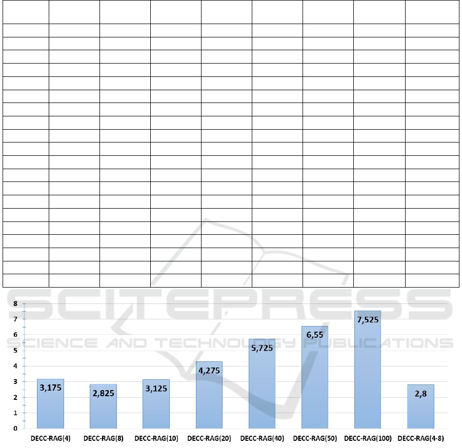
Table 1: The experimental results on the CEC’10 LSGO benchmark problems.

Problem

DECC-

RAG(4)

DECC-

RAG(8)

DECC-

RAG(10)

DECC-

RAG(20)

DECC-

RAG(40)

DECC-

RAG(50)

DECC-

RAG(100)

DECC-

RAG(4-8)

1 7.96E-10 1.02E-17

1.97E-18

3.30E-10 1.61E+02 1.58E+04 1.91E+07 6.55E-14

2 3.00E+03 1.23E+03

7.87E+02

1.82E+03 4.62E+03 5.16E+03 5.85E+03 2.99E+03

3 1.09E+01 2.75E+00 1.49E+00

1.21E-08

1.09E-02 1.45E-01 3.53E+00 1.06E+01

6.85E+11

9.67E+11 1.02E+12 2.24E+12 3.45E+12 4.58E+12 8.99E+12 9.35E+11

5 7.96E+07 1.43E+08 1.63E+08 2.27E+08 3.94E+08 4.86E+08 7.00E+08

7.67E+07

2.03E+01 2.03E+01

2.04E+01 2.07E+01 1.98E+07 2.00E+07 2.00E+07

2.03E+01

7 5.93E+00 8.76E+00 1.70E+02 5.06E+05 1.08E+08 3.39E+08 3.09E+09

2.00E+00

2.09E+04

1.03E+07 2.36E+07 4.07E+07 1.17E+08 1.47E+08 3.01E+08 2.76E+06

4.22E+07

5.46E+07 6.60E+07 1.15E+08 1.97E+08 2.31E+08 3.44E+08 4.40E+07

10 4.98E+03 3.70E+03 3.24E+03

2.11E+03

5.27E+03 8.85E+03 1.17E+04 4.89E+03

1.11E+02

2.15E+02 2.16E+02 2.35E+02 2.35E+02 2.35E+02 2.35E+02 1.15E+02

12 2.73E+04 9.05E+03

8.68E+03

2.51E+04 9.51E+04 1.32E+05 3.34E+05 1.38E+04

13 1.33E+03 1.69E+03

1.30E+03

2.92E+03 1.06E+04 3.32E+04 2.20E+05 2.09E+03

14 1.70E+08 1.70E+08 2.00E+08 4.07E+08 1.09E+09 1.40E+09 3.09E+09

1.61E+08

15 5.78E+03 5.27E+03 5.00E+03

4.32E+03

1.29E+04 1.36E+04 1.53E+04 5.73E+03

16 2.79E+02 4.11E+02 4.28E+02 4.29E+02 4.29E+02 4.29E+02 4.28E+02

2.63E+02

17 2.22E+05

1.46E+05

1.67E+05 3.91E+05 9.90E+05 1.27E+06 1.74E+06 1.80E+05

3.81E+03

4.92E+03 5.95E+03 9.74E+03 1.18E+05 1.07E+05 1.01E+05 5.80E+03

19 1.86E+06 1.98E+06 2.20E+06 4.41E+06 1.29E+07 1.56E+07 1.57E+07

1.68E+06

20 2.29E+03 1.91E+03 1.82E+03 1.13E+03

1.04E+03

1.06E+03 2.97E+03 2.16E+03

Figure 1: The DECC-RAG(m) ranking.

The experimental results for the DECC-RAG(m)

are presented in Table 1. Figure 1 shows the results

of ranking the investigated algorithms (ranks are

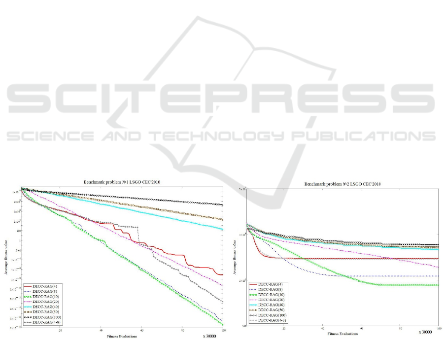
averaged over the benchmark problems). Figures 3-

12 demonstrate the convergence of the best-found

solutions of each algorithm averaged over 25

independent runs.

As we can see from the Table 1, the DECC-RAG

algorithm performs better with small number of

subcomponents, which contains large number of

variables. This means that the approach is able to

provide an efficient decomposition of a problem and

to form efficient combinations of variables in

subcomponents. The best results are achieved by the

DECC-RAG(8), DECC-RAG(4) and DECC-

RAG(10). At the same time, we can see in the

Figures 3-12 that different configurations of the

algorithm have different speeds of the convergence.

Some configurations have good convergence at the

early stages of the search process, but have worse

the best-found value. Some configurations

demonstrate low convergence speed, but are able to

improve the best-found value at the finally stage of

the search process. Thus, we can conclude that the

IJCCI 2018 - 10th International Joint Conference on Computational Intelligence

258

dynamic sizing of subcomponents may improve the

performance of the algorithm.

The DECC-RAG(4-8) is a straightforward

approach of changing the number of subcomponents

during the run of the algorithm. As we can see in the

Figure 1, this configuration has taken the best

average rank over the benchmark.

In real-world LSGO problems, the best settings

for the algorithms are unknown beforehand and the

m value can be chosen at random. Our hypothesis is

that the dynamic sizing is more preferable than the

random choice of m. The performance of the random

choice of m can be estimated by evaluating the

average performance of all configurations. We have

compared the DECC-RAG(4-8) with the following

average values:

 The average of 4 and 8 for establishing the

difference in the performance against the

random choice of m=4 and m=8;

 The average of 4, 8, 10 and 20, because we

have found that lower values of m perform

better;

 The average of 4, 8, 10, 20, 40, 50, 100 for

investigating the random choice of m.

Figure 2 shows the results of ranking the DECC-

RAG(4-8) and the estimated performance of random

choice of m.

Figure 2: Comparison of ranks for the DECC-RAG(4-8)

and the average of DECC-RAG(m).

Table 2 contains the results of Mann–Whitney U

test with p-value equal to 0.05. We use the following

notations in Tables 2: the sign “<” means that the

first algorithm outperforms the second one,

otherwise the sign “>” is used, and the sign “≈” is

used when there is no statistically significant

difference in the results.

As we can see from the results, the dynamic

sizing is more preferable than the random choice

when the optimal value of m is unknown. Also, we

can see from Table 1 that the dynamic sizing

(DECC-RAG(4-8)) is better than the best

configuration of the DECC-RAG(m) with m=8.

It is obvious that the dynamic sizing can be

implemented with other combinations of parameter

m. Moreover, we can use not only deterministic

schemes, but we can change sizes adaptively using a

feedback. We will design and investigate these

approaches in our further works.

Table 2: Results of Mann–Whitney U test for

the DECC-RAG(4-8) vs Average(m).

DECC-RAG (4-8) vs Average (4, 8)

< > > ≈ < ≈ < < < >

< < ≈ < > < ≈ > < ≈

DECC-RAG (4-8) vs Average(4, 8, 10, 20)

< > > < < < < < < >

< < ≈ < > < < ≈ < >

DECC-RAG (4-8) vs Average(4, 8, 10, 20, 40, 50, 100)

< < > < < < < < < <

< < < < < < < < < >

4 CONCLUSIONS

In this study, we have presented the investigation of

tuning the number of subcomponents in the random

adaptive grouping algorithm that combines the ideas

of random dynamic grouping and learning dynamic

grouping for solving LSGO problems. The

experimental results have shown that the algorithm

is able to provide an efficient decomposition of a

problem and to form efficient combinations of

variables in subcomponents, thus performs better

when using subcomponents of larger size. We have

also demonstrated that the dynamic sizing is more

preferable than choosing the number of

subcomponents at random, and the straightforward

scheme DECC-RAG(4-8) outperforms the best

configuration of the DECC-RAG. In our further

works, we will investigate other settings of the

proposed approach and other schemes of the

dynamic sizing of subcomponents.

An Investigation of Parameter Tuning in the Random Adaptive Grouping Algorithm for LSGO Problems

259

ACKNOWLEDGEMENTS

This research is supported by the Ministry of

Education and Science of Russian Federation within

State Assignment № 2.1676.2017/ПЧ.

REFERENCES

Chen, W. et al., 2010. Large-scale global optimization

using cooperative coevolution with variable

interaction learning, in Parallel Problem Solving from

Nature, PPSN XI, Springer, pp. 300–309.

Li, X., Tang, K., Omidvar, M.N., Yang, Zh., Qin, K.,

2013. Benchmark functions for the CEC 2013 special

session and competition on large-scale global

optimization, Technical Report, Evolutionary

Computation and Machine Learning Group, RMIT

University, Australia.

Liang, J.J., Suganthan, P.N., 2005. Dynamic multi-swarm

particle swarm optimizer, in Proceedings - 2005 IEEE

Swarm Intelligence Symposium, SIS 2005, pp. 127–

132.

Liu, J., Tang, K., 2013. Scaling up covariance matrix

adaptation evolution strategy using cooperative

coevolution, in Intelligent Data Engineering and

Automated Learning – IDEAL 2013, pp. 350–357.

Mahdavi, S., Shiri, M.E., Rahnamayan, Sh., 2015.

Metaheuristics in large-scale global continues

optimization: A survey, in Information Sciences, vol.

295, pp. 407–428.

Omidvar, M.N. et al., 2014. Cooperative co-evolution with

differential grouping for large scale optimization,

IEEE Transactions on Evolutionary Computation,

18(3), pp. 378–393.

Potter, M.A., De Jong, K.A., 1994. A cooperative

coevolutionary approach to function optimization,

LNCS, vol. 886, pp. 249–257.

Potter, M.A., De Jong, K.A., 2000. Cooperative

Coevolution: An Architecture for Evolving Coadapted

Subcomponents, Evolutionary Computation, 8(1), pp.

1–29.

Ray, T., Yao, X., 2009. A cooperative coevolutionary

algorithm with correlation based adaptive variable

partitioning, in IEEE Congress on Evolutionary

Computation, 2009 (CEC’09), pp. 983–989.

Sopov, E., 2018. Adaptive Variable-size Random

Grouping for Evolutionary Large-Scale Global

Optimization, in Proceedings of ICSI 2018, LNCS

10941, pp. 1–10.

Vakhnin, A., Sopov, E, 2018. A novel method for

grouping variables in cooperative coevolution for

large-scale global optimization problems, in the 15th

International Conference on Informatics in Control,

Automation and Robotics (ICINCO 2018), pp. 1-8.

Yang, Z., Tang, K., Yao, X., 2007. Differential evolution

for high-dimensional function optimization, in IEEE

Congress on Evolutionary Computation, IEEE CEC

2007, pp. 3523–3530.

Yang, Z., Tang, K., Yao, X. 2008a. Multilevel cooperative

coevolution for large scale optimization, in 2008 IEEE

Congress on Evolutionary Computation, CEC 2008,

pp. 1663–1670.

Yang, Z., Tang, K., Yao, X., 2008b. Self-adaptive

differential evolution with neighborhood search, in

2008 IEEE Congress on Evolutionary Computation,

CEC 2008, pp. 1110–1116.

Yang, Z., Tang, K., Yao, X., 2008c, Large scale

evolutionary optimization using cooperative

coevolution, Information Sciences, 178(15), pp. 2985–

2999.

Figure 3: Convergence of the best found for benchmark problems 1 and 2.

IJCCI 2018 - 10th International Joint Conference on Computational Intelligence

260

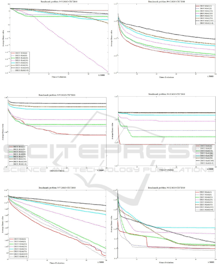
Figure 4: Convergence of the best found for benchmark problems 3 and 4.

Figure 5: Convergence of the best found for benchmark problems 5 and 6.

Figure 6: Convergence of the best found for benchmark problems 7 and 8.

An Investigation of Parameter Tuning in the Random Adaptive Grouping Algorithm for LSGO Problems

261

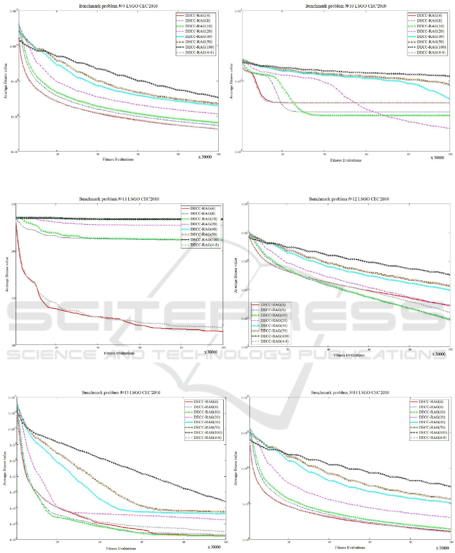
Figure 7: Convergence of the best found for benchmark problems 9 and 10.

Figure 8: Convergence of the best found for benchmark problems 11 and 12.

Figure 9: Convergence of the best found for benchmark problems 13 and 14.

IJCCI 2018 - 10th International Joint Conference on Computational Intelligence

262

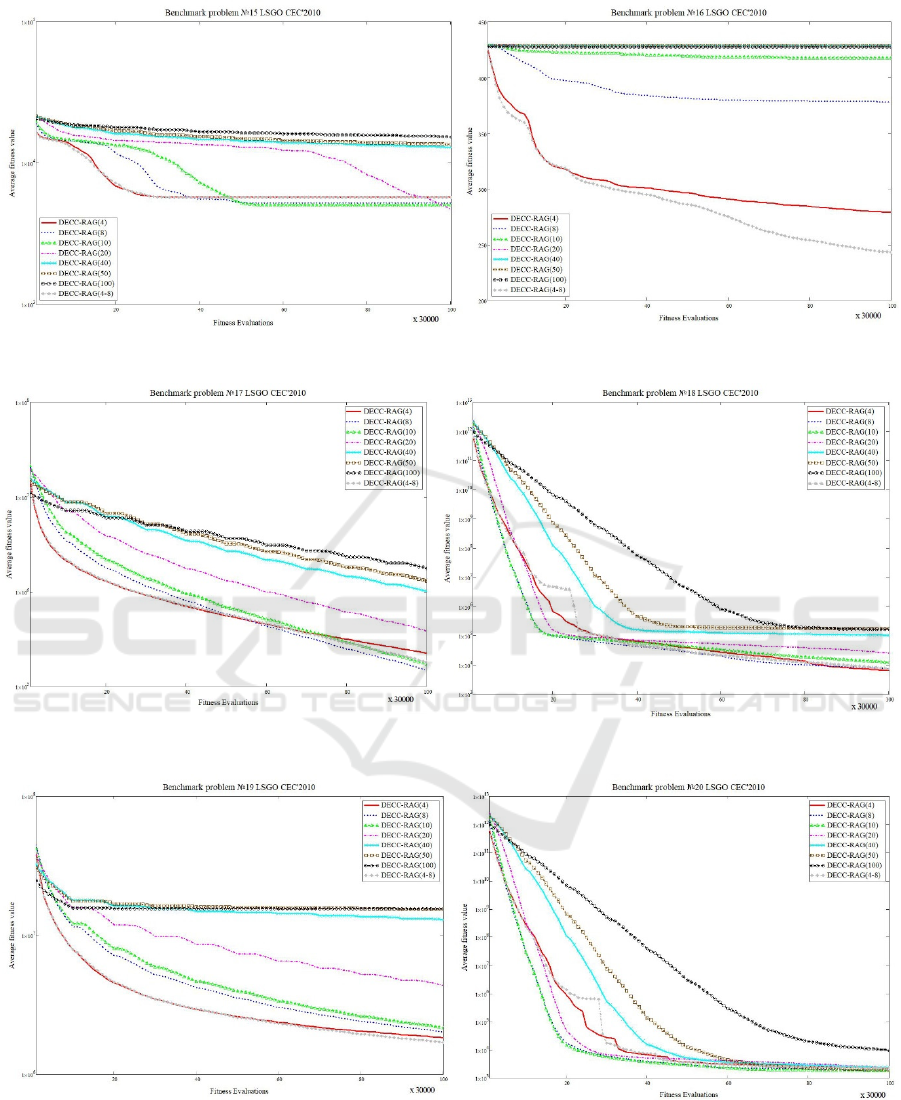
Figure 10: Convergence of the best found for benchmark problems 15 and 16.

Figure 11: Convergence of the best found for benchmark problems 17 and 18.

Figure 12: Convergence of the best found for benchmark problems 19 and 20.

An Investigation of Parameter Tuning in the Random Adaptive Grouping Algorithm for LSGO Problems

263