
Does the Jaya Algorithm Really Need No Parameters?
Willa Ariela Syafruddin
1
, Mario K
¨
oppen
1
and Brahim Benaissa
2
1
Graduate School Creative Informatics, Kyushu Institute of Technology, Fukuoka, Japan
2
Graduate School of Life Science and Systems Engineering, Kyushu Institute of Technology, Fukuoka, Japan
Keywords:
Jaya Algorithm, Swarm Optimization, Benchmark Functions.
Abstract:
Jaya algorithm is a swarm optimization algorithm, formulated on the concept where the solution obtained for a
given problem moves toward the best solution and away from the worst solution. Despite being a very simple
algorithm, it has shown excellent performance for various application. It has been claimed that Jaya algorithm
is parameter-free. Here, we want to investigate the question whether introducing parameters in Jaya might be
of advantage. Results show the comparison of the results for different benchmark function, indicating that,
apart from a few exceptions, generally no significant improvement of Jaya can be achieved this way. The
conclusion is that we have to consider the operation of Jaya differently from a modified PSO and more in the
sense of a stochastic gradient descent.
1 INTRODUCTION
The field of optimization knows a large variety of me-
taheuristic algorithms (Liang et al., 2013), most of
which are inspired from nature, or modifications of
existing algorithms. Jaya algorithm is one of the al-
gorithms proposed by Rao in 2016. Jaya has recently
become popular and found many application cases.
(Rao and Saroj, 2017) proposed an elitist-Jaya algo-
rithm for optimizing the systems amount and functio-
nal amount of shell-and-tube heat exchanger (STHE)
design at the same time. The Jaya algorithm can ef-
ficiently solve optimization problems of diverse ther-
mal systems. (Rao et al., 2016a) proposed dimensi-
onal optimization of a micro-channel heat sink using
Jaya algorithm.The result shows that Jaya algorithm
attains comparable or superior optimal result as rela-
ted to the TLBO and MOE acronyms must be defined
(Warid et al., 2016) presented the Jaya algorithm
to deal with different optimum power flow (OPF) pro-
blems. This algorithm does not need controlling fac-
tors to be tuned.
This algorithm looks structurally very similar to
the Particle Swarm Optimization algorithm, but is de-
signed to be even simpler and without parameters. A
particle in this algorithm, instead heading to the per-
sonal best and the global best simultaneously, it heads
towards the best and away from the worst, and it has
no inertia (Rao, 2016). This behavior is governed by
the following equation:
X
(i+1)
j
= X
(i)
j
+ r
1
·
X
B, j
−
X
(i)
j
−r
2
·
X
w, j
−
X
(i)
j
(1)
Where X
B
is the value of the variable for the best
candidate and X
W
is the value of the variable for the
worst candidate. Once this change of position has a
better objective value, it will replace the former posi-
tion. The three operands in Eq. (1) can also be descri-
bed as: former position plus term of best minus term
of worst. Another difference with the PSO algorithm
is that the best and worst solutions are updated in each
iteration, as opposed to the PSO where the global best
and personal best is updated whenever a better solu-
tion is found(Rao et al., 2016b)(Rao and Patel, 2013).
The Jaya algorithm is described in Fig. 1.
Most of the existing swarm based algorithms have
common controlling parameters, like the number of
particles, or specific parameters like the weight and
global best in the PSO algorithm. The effectiveness of
the optimization is deeply related to the fine tuning of
all parameters. Since the Jaya algorithm requires only
the common control parameters and does not require
any algorithm-specific control parameters, the tuning
is not a requirement. In this work we investigated the
influence of new parameter setting on Jaya algorithm
with doing a parametric study.
This paper is organized as follows. Section 2 pro-
vide some insights on Jaya algorithms and the poten-
tial effect of parameter settings. In Sections 3, we in-
troduce the concept and method we used in this paper.
Section 4 provides result from Jaya algorithm and the
264
Syafruddin, W., Köppen, M. and Benaissa, B.
Does the Jaya Algorithm Really Need No Parameters?.
DOI: 10.5220/0006960702640268
In Proceedings of the 10th International Joint Conference on Computational Intelligence (IJCCI 2018), pages 264-268
ISBN: 978-989-758-327-8
Copyright © 2018 by SCITEPRESS – Science and Technology Publications, Lda. All rights reserved

!"#$#%&#'()*+*, &%$#+")-#'(.)",/0(1)+2)3(-#4"
5%1#%0&(-)%"3)$(1/#"%$#+")61#$(1#+"
!3("$#27)best%%"3)worst%-+&,$#+"-) #")$8(
*+*,&%$#+"
9+3#27)$8()-+&,$#+"-)0%-(3)+")best%%"3)worst%-+&,$#+"-
Xj
(i+1)
:)Xj
(i)
;)r1
・
<X
best,j
= >Xj
(i)
>?)@ r2
・
<X
worst,j
= >Xj
(i)
>?
!-)$8()-+&,$#+")6+11(-*+"3#"4)$+)X'j,k,i
0($$(1)$8%")$8%$)6+11(-*+"3#"4)$+)Xj,k,i ?
A+
B((*)$8()*1(5#+,-
-+&,$#+"
C(-
D66(*$)%"3)1(*&%6(
$8()*1(5#+,-)-+&,$#+"
E(*+1$)$8()+*$#/,/)-+&,$#+"
!-)$8()$(1/#"%$#+")61#$(1#+")-%$# -2#(3F
C(-
A+
Figure 1: Flowchart of the Jaya algorithm proposed by Rao
in 2016.
potential effect of parameter setting that give raise to
related experiments. Then, Section 5 will further re-
fine the experimental study and present our views on
the (rather unexpected) results that we got.
2 SOME INSIGHTS INTO THE
JAYA ALGORITHM
As mentioned above already, it has been pointed out
more than once that the Jaya algorithm is parameter-
free. Up to our knowledge there is no published study
showing if that’s truly the case. In this work we in-
vestigate if there are ways of improving Jaya by intro-
ducing parameters hidden in the original formulation.
We also give a theoretical argument why the use of
such hidden parameters can be of advantage.
Consider an objective function which is best des-
cribes by the metaphor “island in the middle of a
lake.” What we mean is a real-valued function defi-
ned over R and two range values a and b. For |x| > a
we set f (x) = 1, for a ≥ |x| ≥ b we set f (x) = 1000
and for |x| < b we set f (x) = 2. With regard to the
metaphor, the first case is the mainland, providing the
absolute minimum of the function, the second part the
lake, with worse objective values, and surrounding the
island of third case, technically a local optimum. And
in this case, we considering minimization problem.
Considering the Jaya algorithm’s update equation,
Eq. (1) it can be seen that the magnitude of change is
within intra-population distances. The change in the
x position can be at most the largest difference bet-
ween any coordinate of any individual. But then, the
modified x-position is only updated if there is an im-
provement in the objective function values (compared
to PSO, Jaya doesn’t have inertia). It means if we
choose a small b (small island, say b = 1) and large a
(far away from mainland, say a = 100) and also assu-
ming that the initialization of Jaya happened such that
all individuals are located on the island, there will be
never a probe of a position far enough from the island
to reach the mainland. In all cases it will be |x | ≤ 2
and f (x) either 2 or 1000, no x will ever reach an op-
timum position with |x| > a. Thus, Jaya will become
stuck on the island.
Now, introducing parameters here could help, be
it even in a theoretical and impractical way. For ex-
ample, consider the case where weights are added in
Eq. (1) for the repulsion term. If we select a weight
large enough it can be sufficient to probe x values of
|x| > a. Of course, we can also set a range parameter
for r
1
, r
2
with same effect. This is a purely theoretical
argument and we can’t say much how this can influ-
ence Jaya’s performance when applied to real-world
problems or test functions. A series of experiments,
reported on next, has been conducted to see the influ-
ence of weighting parameters on the performance.
The second insight is about the deviation of Jaya
Eq. (1) from a pure vector notation. We mean the
use of |X
i
j
| in the Jaya update rule instead of just X
i
j
.
In the latter case, it would describe a vector pointing
away the worst or towards the best. By using the ab-
solute, and once there is a mixture of positive and
negative component values, the change of an indivi-
dual vector becomes a rather unpredictable issue. So
far, we could not find any explanation or considera-
tion about the choice of the absolute value, but given
the Jaya’s result on various applications from litera-
ture, it doesn’t seem to be a drawback. Therefore, it is
also interesting to see what happens if we select other
functions here instead of the absolute value.
In this work, we conduct a series of experiments to
investigate the influence of hidden parameter settings
on Jaya performance, namely:
• weights for the first and second update term,
• ordered-weights for also taking second-worst and
second-best into account, and
• variants of the coordinate function.
3 EXPERIMENTAL PLAN
3.1 Concept
We wanted to investigate the simple by yet efficient
equation of Jaya, based on both best and worst so-
lutions simultaneously, more specifically we wanted
to see which one of the two is the most effective on
the optimization process, so we introduced weights,
Does the Jaya Algorithm Really Need No Parameters?
265

notices that there should be equal amount of weight
in both best and worst sides. Then finally investiga-
ted the effect of second best and second worst, which
gave good impression on how the algorithm works .
In this study, we tested two things: changing weig-
hts for best and worst, and changing weights by in-
cluding second best and second worst. The algorithm
performance is tested by implementing 12 unconstrai-
ned benchmark functions. The result will directly
show the influence of parameter settings on the per-
formance.
3.2 Method
1. On the first test we used two different weights (1
0 2), (2 0 1), and compare with Jaya algorithm
result. The 0 in the middle stands for the central
group of solutions, i.e. the first weight is for the
best, the third for the worst, all other are 0. From
the original equation (1) we transformed mathe-
matical expression as
X
(i+1)
j
= X
(i)
j
+ 1 · r
1
·
X
B, j
−
X
(i)
j
− 2 ·r
2
·
X
w, j
−
X
(i)
j
(2)
X
(i+1)
j
= X
(i)
j
+ 2 · r
1
·
X
B, j
−
X
(i)
j
− 1 ·r
2
·
X
w, j
−
X
(i)
j
(3)
2. For the second test we used five different weights:
(0.9 0.1 0 -0.1 -0.9), (0.7 0.3 0 -0.3 -0.7), (0.5 0.5
0 -0.5 -0.5), (0.3 0.5 0 -0.5 -0.3), and (0.8 0 0 0
-0.8). Same here regarding notation, in addition
weights for second best and worst are introduced
as follows:
X
(i+1)
j
= X
(i)
j
+ 0.9 · r
1
·
X
B1, j
−
X
(i)
j
+ 0.1 · r
2
·
X
B2, j
−
X
(i)
j
− 0.1 ·r
2
·
X
w1, j
−
X
(i)
j
− 0.9 ·r
2
·
X
w2, j
−
X
(i)
j
(4)
X
(i+1)
j
= X
(i)
j
+ 0.7 · r
1
·
X
B1, j
−
X
(i)
j
+ 0.3 · r
2
·
X
B2, j
−
X
(i)
j
− 0.3 ·r
2
·
X
w1, j
−
X
(i)
j
− 0.7 ·r
2
·
X
w2, j
−
X
(i)
j
(5)
X
(i+1)
j
= X
(i)
j
+ 0.5 · r
1
·
X
B1, j
−
X
(i)
j
+ 0.5 · r
2
·
X
B2, j
−
X
(i)
j
− 0.5 ·r
2
·
X
w1, j
−
X
(i)
j
− 0.5 ·r
2
·
X
w2, j
−
X
(i)
j
(6)
X
(i+1)
j
= X
(i)
j
+ 0.3 · r
1
·
X
B1, j
−
X
(i)
j
+ 0.5 · r
2
·
X
B2, j
−
X
(i)
j
− 0.5 ·r
2
·
X
w1, j
−
X
(i)
j
− 0.3 ·r
2
·
X
w2, j
−
X
(i)
j
(7)
X
(i+1)
j
= X
(i)
j
+ 0.8 · r
1
·
X
B, j
−
X
(i)
j
− 0.8 ·r
2
·
X
w, j
−
X
(i)
j
(8)
We used 12 test functions as shown in Table 1 and
their selection is based on two facts: (1) usually they
are part of other benchmark function sets, but (2) also
that the goal is not to propose an absolute best algo-
rithm but to directly compare the influence of para-
meter settings on the performance. Result obtained
by the Jaya algorithm for 25 population with 500000
maximum fitness evaluation.
4 RESULT
Results for Method 1 the first used three different
weights are shown in Table 2. Note as this were initial
experiments, the selection of functions is a bit diffe-
rent than for the main experiment. Apart from two
functions, there is no gain but a loss is rather likely.
We can’t find any notable way of improving Jaya this
way.
Table 3 shows dimension result from benchmark
functions where Weight1 is (0.9 0.1 0 -0.1 -0.9) equa-
tion (4), the choice of weights (including second best
attraction and second worst repulsion terms) is accor-
ding to Method 2. We can see from Figure 2 graphic
one of unconstrained benchmark function is Beale
function that contains five different weight.
We also calculated the 95% significance levels for
the results shown in Table 3: first weight (0,9 0,1 0
-0,1 -0,9) the p-value= 0.1875, means in this case not
significantly better (a bit better only), while for other
weights ((0.7 0.3 0 -0.3 -0.7),(0.5 0.5 0 -0.5 -0.5),(0.3
0.5 0 -0.5 -0.3),(0.8 0 0 0 -0.8)) the p-value= 0.0625,
is mean in this case Jaya with standard parameter set-
ting is significantly better than Jaya with other para-
meter settings because normally p-value= 0.05 and it
is close to 0.0625 as shown in Table 4.
IJCCI 2018 - 10th International Joint Conference on Computational Intelligence
266
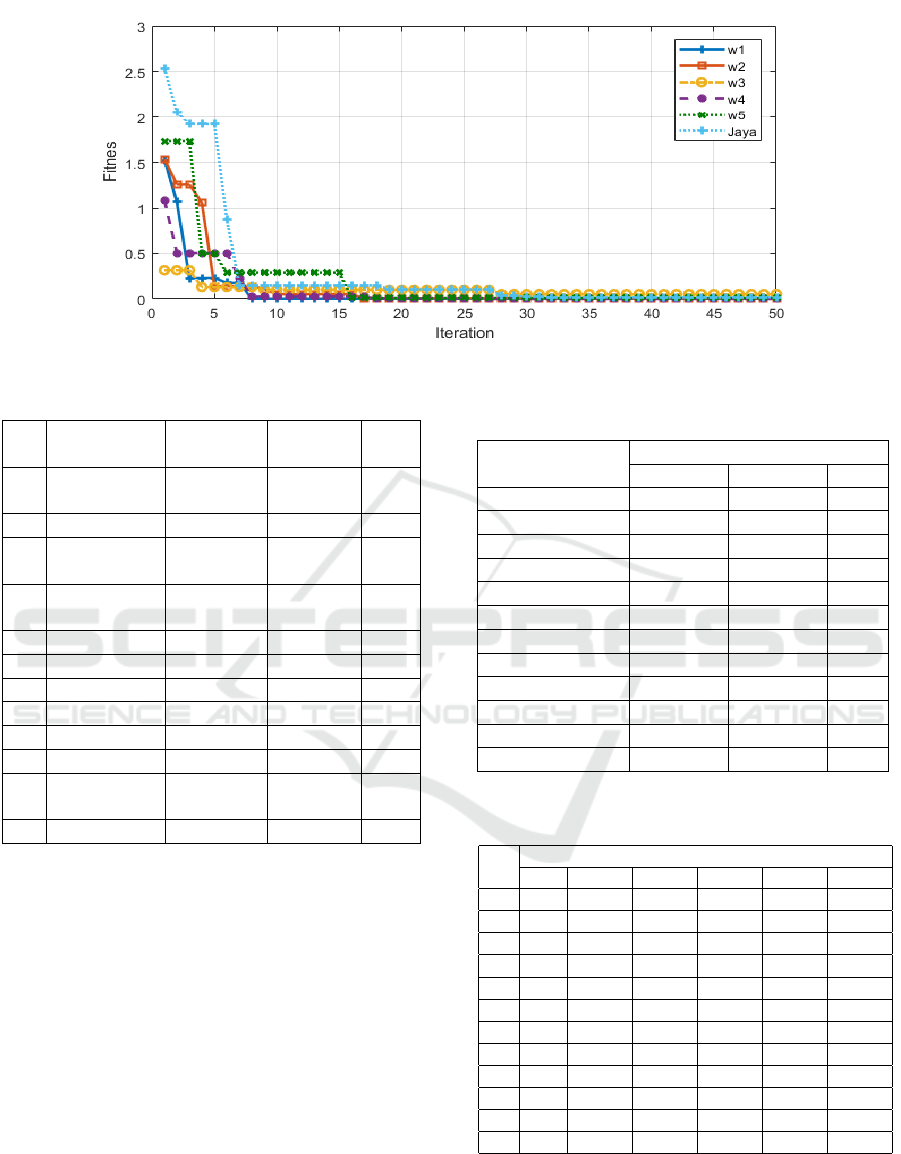
Figure 2: Fitness convergence in the case of Beale function with five different ordered weights.
Table 1: Unconstrained Benchmark Functions.
F Function Dimension Search
Range
C
F1 Sphere 30 [-100,
100]
US
F2 SumSquares 30 [-10, 10] US
F3 Beale 5 [-4.5,
4.5]
UN
F4 Easom 2 [-100, -
100]
UN
F5 Matyas 2 [-10, 10] UN
F6 Colville 4 [-10,10] UN
F7 Zakharov 10 [-5, 10] UN
F8 Rosenbrock 30 [-30, 30] UN
F9 Branin 2 [-5,10] MS
F10 Booth 2 [-10, 10] MS
F11 GoldStein-
Price
2 [-2, 2] MN
F12 Ackley 30 [-32, 32] MN
F:Function C: Characteristic U: Unimodal, M: Multimo-
dal, S: Separable, N: Non-separable.
5 DISCUSSION AND OUTLOOK
The experimental result of this research shows that
Jaya still works best without weighting parameters for
most functions. After experimenting with different
weight values, the research perspective about Jaya be-
came more evident. Furthermore, to get better insight
on how the weights are affecting the search in Jaya
process, the fitness convergence plots are compared
and analyzed extensively.
This way we can see how quickly stagnation will
occur (stuck in local minima, or not being able to find
better solutions because of too scattered search). As
mentioned before in this research, to see the result
Table 2: Result Obtained by The Jaya Algorithm with Three
Different Weight.
Function Standard Deviation
(102) (201) Jaya
Sphere 0 0 0
SumSquares 0 308.28 0
Beale 0 0 0
Easom 0 0 0
Matyas 0 0 0
Colville 0 0 0
Zakharov 0.00364 0.000033 0
Rosenbrock 0.000014 8888003 0
Branin 0 0 0
Booth 0 0 0
GoldStein-Price 0.000008 0.000007 0
Ackley 0.045268 0.001646 0
Table 3: Result Obtained by The Jaya Algorithm with Five
Different Weight.
F Dimension
Jaya W1 W2 W3 W4 W5
F1 0 0 0 0 0 0
F2 0 0 0 0 0 0
F3 0 0.34 0.0009 0.015 0.0084 0.0008
F4 0 0 0.19 0 0.0002 0
F5 0 0 0 0 0 0
F6 0 0 0.52 0.45 1.13 1.38
F7 0 0 0 0 0 0
F8 0 0 1647.1 7.97 0 0.88
F9 0 0.0003 0.0053 0.0063 0.0008 0.001
F10 0 0 0 0 0 0
F11 0 0.012 0 0.106 0.012 0
F12 0 0.81 0 0 0 0.42
from a different perspective, some part of the Jaya
formula is modified. The first modification is to try
the formula without absolute value (abs) for Booth
function, and this modification resulted in the follo-
Does the Jaya Algorithm Really Need No Parameters?
267

Table 4: Test on Statistical Significance for Beale Function
using Wilcoxon Signed-Rank Test.
Weight V P-Value
(0.9 0.1 0 -0.1 -0.9) 2 0.1875
(0.7 0.3 0 -0.3 -0.7) 0 0.0625
(0.5 0.5 0 -0.5 -0.5) 0 0.0625
(0.3 0.5 0 -0.5 -0.3) 0 0.0625
(0.8 0 0 0 -0.8) 0 0.0625
Table 5: Modified Jaya Formula used Beale Function.
Function Best Worst Mean SD
Square 0 0.000003 0.000001 0.000001
Log 0 0.000006 0.000002 0.000002
Sin 0 0 0 0
SD: Standard Deviation.
wing best = 0, worst = 0.000001, mean = 0, and stan-
dard deviation = 0. Even using sinus as coordinate
function, we can get a good result. We try in Beale
function too as shown in Table 5 and get a good result
too.
A further study might be needed to investigate the
influence of this coordinate functions, as it seems to
be able to improve the performance in some cases.
But it also poses the question on how we understand
the working of this seemingly simple and nice algo-
rithm. The findings reported here give a clear indi-
cation that Jaya is not a PSO variant. Not only that
it differs from a PSO in structural aspects (no inertia,
no reference to vector operations), also the initial sta-
tement “towards the best and away from the worst”
might not tell the whole story. Our proposal here is
to understand Jaya more in the sense of a stochas-
tic gradient/anti-gradient based search. All these al-
ternative coordinate functions have in common that
their average value is related to the coordinate va-
lue of an individual, while there are random fluctu-
ations around this value. In the common gradient-
descent learning method, the search goes into the di-
rection of strongest change of objective function va-
lue. Here, we can find a composition of this direction
with the opposite direction of strongest loss (dubbed
anti-gradient right now). Further investigations are
needed to see how much this gives the better picture,
and means for understanding and planning Jaya appli-
cation in practice (as well as the design of other algo-
rithms, or modification of known algorithms in same
sense).
6 CONCLUSION
As mentioned in Rao Journal (2015) about Jaya algo-
rithm not require any algorithm-specific control para-
meters, the experiment result of this research shows
that Jaya still works best weighting parameters too.
In this paper, we tested two things: changing weights
for best and worst, and changing weights by including
second best and second worst.
We proposed seven different weight and tested the
algorithm performance by implementing 12 uncon-
strained benchmark function. From the result we can
understand about Jaya algorithm is more in the sense
of stochastic gradient/anti-gradient based search.
REFERENCES
Liang, J., Qu, B., and Suganthan, P. (2013). Problem de-
finitions and evaluation criteria for the cec 2014 spe-
cial session and competition on single objective real-
parameter numerical optimization. Computational In-
telligence Laboratory, Zhengzhou University, Zhengz-
hou China and Technical Report, Nanyang Technolo-
gical University, Singapore.
Rao, R. (2016). Jaya: A simple and new optimization algo-
rithm for solving constrained and unconstrained op-
timization problems. International Journal of Indus-
trial Engineering Computations, 7(1):19–34.
Rao, R., More, K., Taler, J., and Ocło
´
n, P. (2016a). Di-
mensional optimization of a micro-channel heat sink
using jaya algorithm. Applied Thermal Engineering,
103:572–582.
Rao, R., More, K., Taler, J., and Ocło
´
n, P. (2016b). Di-
mensional optimization of a micro-channel heat sink
using jaya algorithm. Applied Thermal Engineering,
103:572–582.
Rao, R. and Patel, V. (2013). Comparative performance
of an elitist teaching-learning-based optimization al-
gorithm for solving unconstrained optimization pro-
blems. International Journal of Industrial Engineer-
ing Computations, 4(1):29–50.
Rao, R. V. and Saroj, A. (2017). Constrained economic
optimization of shell-and-tube heat exchangers using
elitist-jaya algorithm. Energy, 128:785–800.
Warid, W., Hizam, H., Mariun, N., and Abdul-Wahab, N. I.
(2016). Optimal power flow using the jaya algorithm.
Energies, 9(9):678.
IJCCI 2018 - 10th International Joint Conference on Computational Intelligence
268
