Low Level Big Data Compression
Jaime Salvador-Meneses
1
, Zoila Ruiz-Chavez
1
and Jose Garcia-Rodriguez
2
1
Universidad Central del Ecuador, Ciudadela Universitaria, Quito, Ecuador
2
Universidad de Alicante, Ap. 99. 03080, Alicante, Spain
Keywords:
Big Data, Data Compression, Categorical Data, Encoding.
Abstract:
In the last years, some specialized algorithms have been developed to work with categorical information, ho-
wever the performance of these algorithms has two important factors to consider: the processing technique
(algorithm) and the representation of information used. Many of the machine learning algorithms depend on
whether the information is stored in memory, local or distributed, prior to processing. Many of the current
compression techniques do not achieve an adequate balance between the compression ratio and the decom-
pression speed. In this work we propose a mechanism for storing and processing categorical information by
compression at the bit level, the method proposes a compression and decompression by blocks, with which
the process of compressed information resembles the process of the original information. The proposed met-
hod allows to keep the compressed data in memory, which drastically reduces the memory consumption. The
experimental results obtained show a high compression ratio, while the block decompression is very efficient.
Both factors contribute to build a system with good performance.
1 INTRODUCTION
Machine Learning (ML) algorithms work iteratively
on large datasets using read-only operations. To get
better performance in the process, it’s important to
keep all the data in local or distributed memory (Elgo-
hary et al., 2017), these methods base their operation
on classical techniques that become complex when
the amount of data increases considerably (Roman-
gonzalez, 2012).
The reduction of the execution time is an impor-
tant factor to work with Big Data which demands
a high consumption of memory and CPU resources
(Hashem et al., 2016). Some ML algorithms have
been adapted to work with categorical data. This is
the case of fuzzy-kMeans that was adapted to fuzzy-
kModes (Huang and Ng, 1999) to work with catego-
rical data (Gan et al., 2009).
Nowadays, it is a challenge to process data sets
with a high dimensionality such as the census carried
out in different countries (Rai and Singh, 2010). A
census is a particularly relevant process and currently
constitutes a fundamental source of information for a
country (Bruni, 2004).
This work proposes a new method to represent and
store categorical data through the use of bitwise ope-
rations. Each attribute f (column) is represented by a
one-dimensional vector.
The method proposes to compress the informa-
tion (data) into packets with a fixed size (16, 32, 64
bits), in each packet a certain amount of values (data)
is stored through bitwise operations. Bitwise opera-
tions are widely used because they allow to replace
arithmetics operations with more efficient operations
(Seshadri et al., 2015). The validity of the method has
been tested on a public dataset with good results.
This document is organized as follows: Section 2
summarizes the representation of the information
and the categorical data compression algorithms, in
Section 3 an alternative is presented for the represen-
tation of information by compression using bitwise
operations, Section 4 presents several results obtained
using the proposed compression method and, finally,
Section 5 summarizes some conclusions.
2 COMPRESSION ALGORITHMS
The main goal of this work is the compression of cate-
gorical data, so in this section we present a summary
of some methods for the compression of categorical
data.
Categorical data is stored in one-dimensional vec-
tor or in matrix composed by vectors depending on
Salvador-Meneses, J., Ruiz-Chavez, Z. and Garcia-Rodriguez, J.
Low Level Big Data Compression.
DOI: 10.5220/0007228003530358
In Proceedings of the 10th International Joint Conference on Knowledge Discovery, Knowledge Engineering and Knowledge Management (IC3K 2018) - Volume 1: KDIR, pages 353-358
ISBN: 978-989-758-330-8
Copyright © 2018 by SCITEPRESS – Science and Technology Publications, Lda. All rights reserved
353

the information type. Matrix representation uses the
vectorial representation of its rows or columns so it
is useful to describe the storage using rows and co-
lumns.
The following describes some options of compres-
sion and representation of one-dimensional data sets
(vectors).
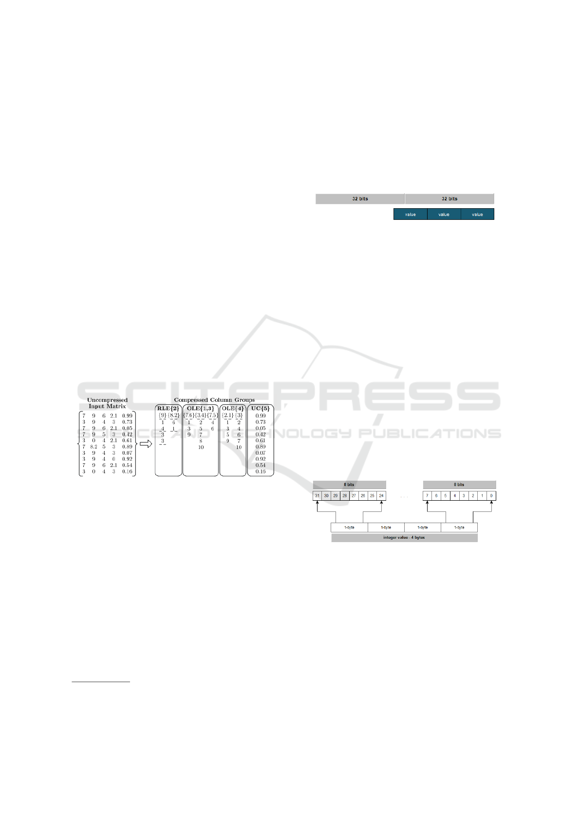
Run-length Encoding: Consecutive sequences of
data with the same value are stored as a pair
(count,value) in which value represents the value to
be represented and count represents the number of
occurrences of the value within the sequence.
There are variations to this type of representation
in which if the sequence of equal values are repea-
ted in different position of the vector, the value is sto-
red and additional to this, the beginning and the total
number of elements in each sequence are represented
(Elgohary et al., 2016).
Offset-list Encoding: For each distinct value within
the data set a new list is generated which contains the
indexes in which the aforementioned value appears.
In the case that there are two correlated set, a (x,y)
pair is generated and the index in which the data pair
appears is stored in the new list.
Figure 1 shows Run-Length encodig (RLE) and
Offset-list encoding (OLE) compression schemas.
Figure 1: Compression examples (Elgohary et al., 2017).
GZIP: Compression is based in the DEFLATE algo-
rithm
1
that consists in two parts: Lz77 and Huffman
coding. The Lz77 algorithm compress the data remo-
ving redundant parts and the Huffman coding codes
the result generated by Lz77 (Ouyang et al., 2010).
The classical compression methods, such as GZIP,
considerably overloads the CPU which minimizes the
performance gained by reducing the read/write ope-
rations, this fact makes them unfeasible options to be
implemented in databases (Chen et al., 2001).
Bit Level Compression: REDATAM software
2
uses
a distinct data compression schema that is based in 4-
bytes blocks. Each block stores one or more values
depending of the maximum size in bits required to
store the values (De Grande, 2016).
1
https://tools.ietf.org/html/rfc1952
2
http://www.redatam.org
This compression format represents the most vi-
able option when working with categorical data, be-
cause in most cases the information to be represen-
ted has a low number of different categories. This
method uses the total amount of available bits in each
block, so that a value can be contained in two diffe-
rent blocks of compressed data. Figure 2 shows the
above.
Figure 2: REDATAM compression.
3 COMPRESSION APPROACH
In this section we propose a new mechanism for com-
pressing categorical data, the compression method
proposal corresponds to a variation of the bit level
compression method described in Section 2. This
method doesn’t use all available bits because 32 may
not be a multiple of the number of bits needed to re-
present the categories.
The numerical information of categorical varia-
bles is represented, traditionally, as signed integer va-
lues of 32, 16 or 8 bits (4, 2, 1 bytes). This implies
that to store a numerical value it is necessary to use 32
bits (or its equivalent in 2 or 1 byte). We will consider
the case in which the information is represented as a
set of 4-bytes integer values.
Figure 3 represents the bit distribution of a integer
value composed of 4 bytes.
Figure 3: Representation of an integer value - 4 bytes.
There are variations to the representation showed
in Figure 3 due to the integer values can be represen-
ted in Little Endian or Big Endian format.
If the original variable has m observations, the size
in bytes needed to represent all the observations (wit-
hout compression) is: Total bytes = T b = m ∗ 4
If we consider that all 32 bits are not used to re-
present the values, there is a lot of wasted space.
In Figure 4, the gray area corresponds to space that
is not used. Out of a total of 4 ∗32 = 128 bits, only 16
are used, which represents 12.5% of the total storage
used.
KDIR 2018 - 10th International Conference on Knowledge Discovery and Information Retrieval
354

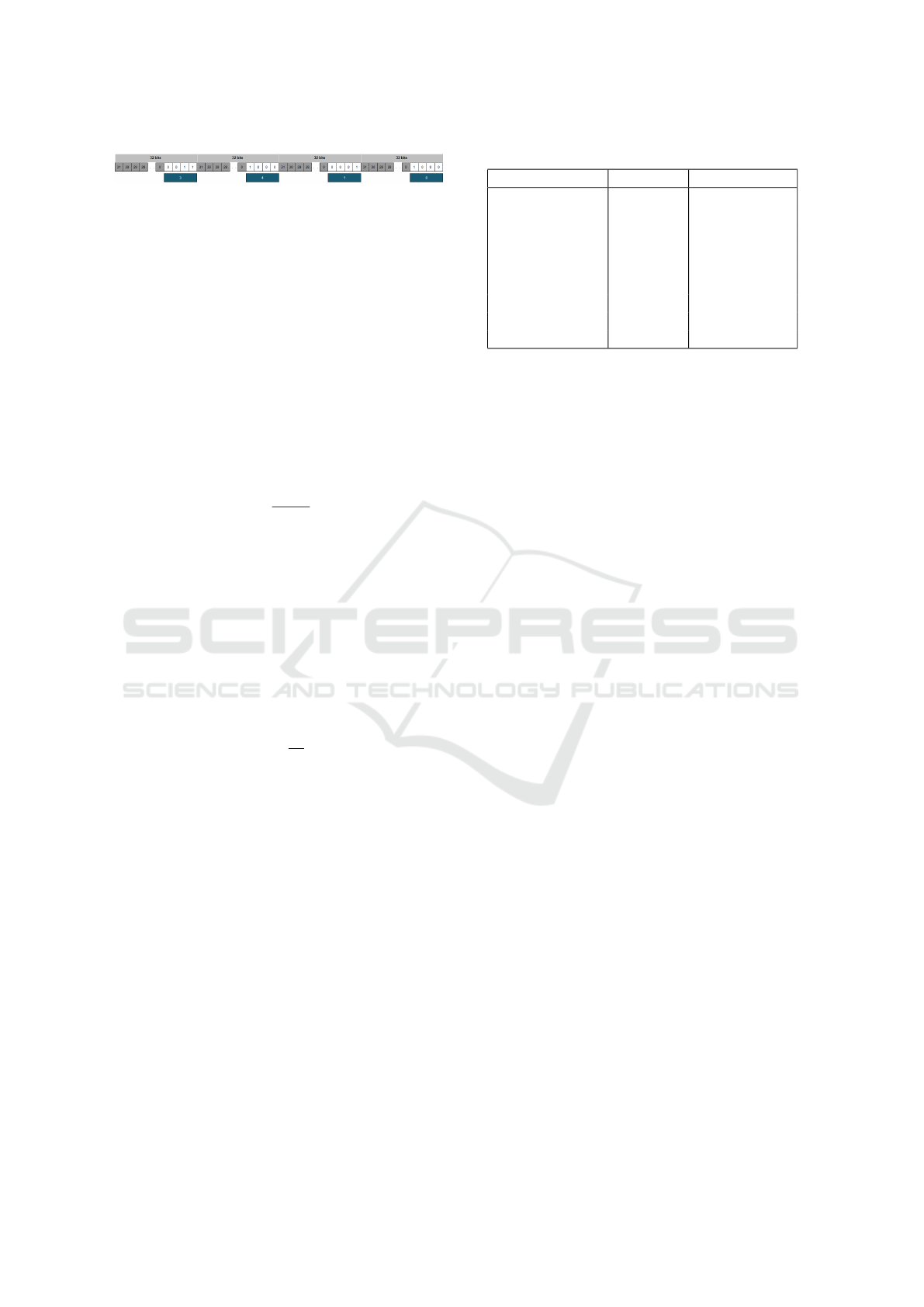
Figure 4: Example, representation of 4 values.
The central idea of this work consists in re-use the
gray areas.
3.1 Minimum Number of Bits
Let V = {v
1
,v
2
,v
3
,...,v
m−1
,v
m
} a categorical varia-
ble where the values v
i
∈ D = {x
1
,x
2
,x
3
,...,x
k
} (set
of all possible values that variable V may take). It is
required that the values of the set D are ordered from
lowest to highest, this is x
1
< x
2
< x
3
< ... < x
k
. From
the previous definition, the values of a categorical va-
riable are between x
1
and x
k
.
The minimum number of bits needed to represent
a value of the aforementioned variable corresponds to:
n =
l
ln(x
k
)
ln(2)
m
(1)
where d·e represents the smallest integer greater
than or equal to its argument and is defined by dxe =
min{p ∈ Z|p > x}.
3.2 Maximum Number of Values
Represented
Using Equation (1), we can determine the number of
elements of the V variable that can be stored within
an integer value (4 bytes):
N
V
=
j
32
n
k
(2)
where b·c represents the largest integer less than or
equal to its argument and is defined by bxc = max{p ∈
Z|p 6 x}.
With this solution it is possible that 32 bits were
not used in total, leaving a number of these unused.
Table 1 shows a summary of the number of bits
used to represent a certain number of categories. The
first column shows the number of categories to repre-
sent (2, between 3 and 4, between 5 and 8, etc.), the
second column shows the number of bits needed to
represent the categories mentioned, finally the third
column shows the total number of elements that can
be represented within 32 bits.
This method generates a new subset V
0
that con-
tains integer values, which in turn contain N
V
ele-
ments of the original set. The number of elements
in this set is given by:
Number o f elements = m/N
v
(3)
Table 1: Amount of elements to represent.
Num. categories Num. bits Total elements
2 1 31
3 to 4 2 15
5 to 8 3 10
9 to 16 4 7
17 to 32 5 6
33 to 64 6 5
65 to 128 7 4
129 to 256 8 3
257 to 512 9 3
where m is the number of elements of the original set
V and N
V
is given by Equation (2).
3.3 Indexing Elements
To index an element within the original set V , it is
necessary to double indexing the set V
0
. Let i be the
index of the element to be searched within the original
set V , the index i
0
on the set V
0
is given by:
p = bi/N
v
c ; q = i mod N
v
(4)
which represents the index on the 32-bit element
to determine the actual value sought.
In summary, the element of the i-th position in the
set V can be extracted from the set V
0
in the following
way:
v
i
= (V
0
p
 q ∗ n) & mask (5)
where p and q are given by the Equation (4) and
mask = 111...1 (sequence of n values 1, n is given by
the Equation (1)). Figure 5 illustrates the above.
3.4 Algorithms
The algorithm represents n categorical values of a va-
riable within 4-bytes. This means that to access the
value of a particular observation, a double indexing
is necessary: access the index of the integer value (4-
bytes) that contains the searched element and next in-
dex within 32 bits to access the value.
The implementation of the proposed method uses
a mixture of arithmetic operations and bitwise ope-
rations: Logical AND (&), Logical OR (|), Logical
Shift Left (), Logical Shift Right ().
Algorithm 1 represents the algorithm to compress
a traditional vector to the bit-to-bit format and algo-
rithm 2 represents the algorithm to iterate over a com-
pressed vector.
Low Level Big Data Compression
355

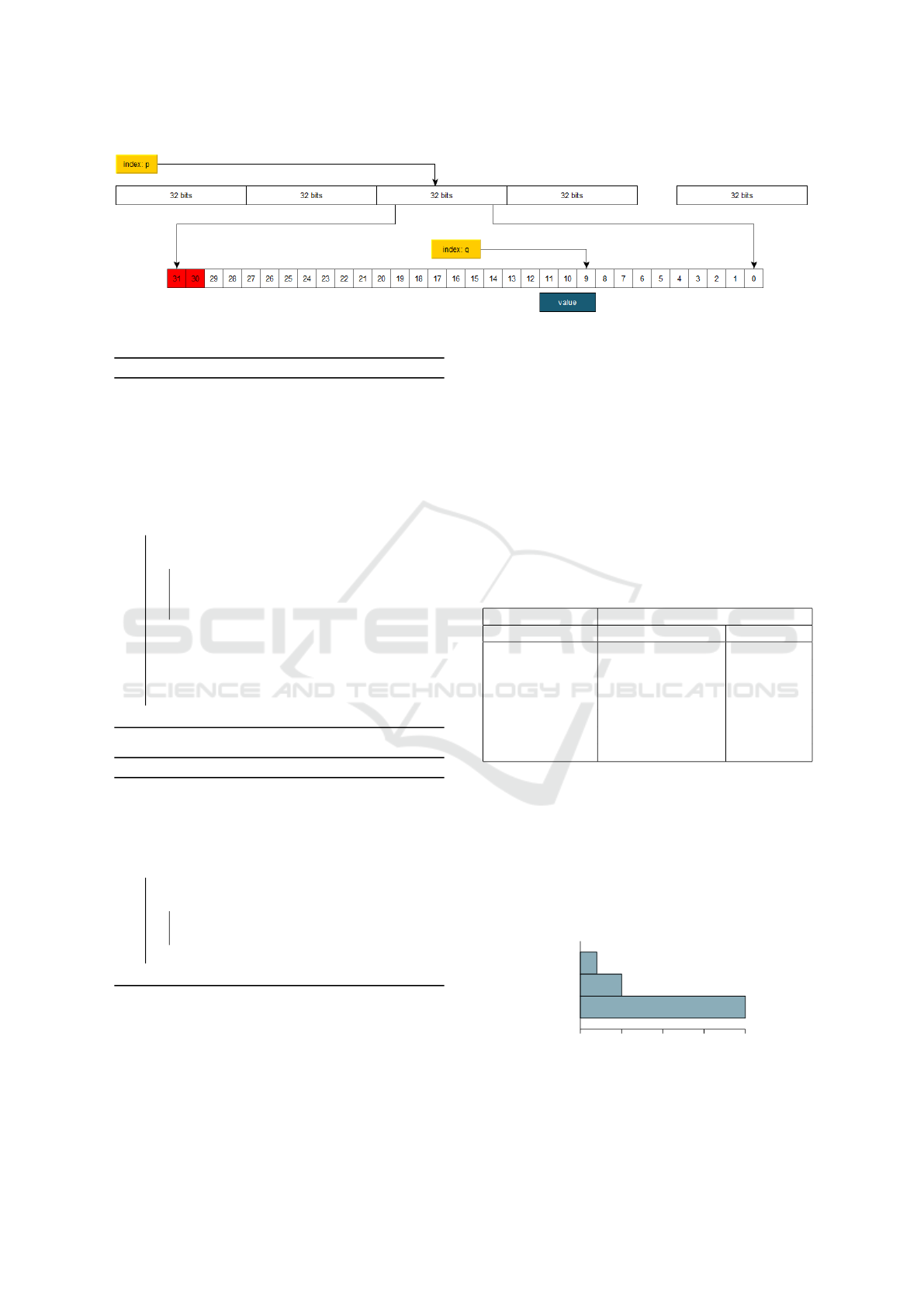
Figure 5: Indexing elements.
Algorithm 1: Compression algorithm.
Data: data, size, dataSize
Result: buffer, buferSize, elementsPerBlock
1 elementsPerBlock ← 32/dataSize;
2 bu f f erSize ← ceil(size/elementsPerBlock);
3 bu f f er ← new int[bu f f erSize];
4 blockCounter ← 0;
5 elementCounter ← 0;
6 for i ← 0 to size − 1 do
7 value ← data[i];
8 if blockCounter ≥ elementsPerBlock then
9 blockCounter ← 0;
10 elementCounter ←
elementCounter + 1;
11 end
12 vv ← value  (dataSize ∗ blockCounter);
13 bu f f er[elementCounter] ←
bu f f er[elementCounter] | vv;
14 blockCounter ← blockCounter + 1;
15 end
Algorithm 2: Iteration algorithm.
Data: vector, size, dataSize
1 elementsPerBlock ← 32/dataSize;
2 mask ← sequence of dataSize-bits with value
= 1
3 for index ← 0 to size − 1 do
4 value ← vector[index];
5 for i ← 0 to elementsPerBlock − 1 do
6 v ← (valor  i ∗ dataSize) & mask;
7 do something with v;
8 end
9 end
4 EXPERIMENTS
This section presents the result of the compression of
random generated vector and some known datasets.
The memory consumption of the representation of the
data in the main memory of a computer was analyzed,
this value represents the amount of memory necessary
to represent a vector of n-elements.
4.1 Random Vectors
In the first instance, several vectors of size 10
3
,
10
4
,..., 10
9
elements were generated. The test data
set contains elements randomly generated in the range
[0,120].
Table 2 shows the result of compressing different
vectors using the proposed method.
Table 2: Memory consumption.
Memory consumption (Kb)
Size (# elements) Uncompressed (int) Compressed
10
3
3.9 1
10
4
3.9 ∗ 10
1
10
1
10
5
3.9 ∗ 10
2
10
2
10
6
3.9 ∗ 10
3
10
3
10
7
3.9 ∗ 10
4
10
4
10
8
3.9 ∗ 10
5
10
5
10
9
3.9 ∗ 10
6
10
6
For the following tests we considered a vector of
size n = 10
9
whose elements are integer values in the
range of 0 to 120. The representation of each element
corresponds to a 32-bit floating value, whereby the
size in bytes to represent the vector is total bytes =
10
9
∗ 4 bytes. This value represents 100% in the Fi-
gure 6 which shows the memory consumption for the
vector representation mentioned above and the repre-
sentation by 7 bits and 2 bits.
10%
2 bit by bit
25%
7 bit by bit
100%
Float vector
0% 25% 50% 75% 100%
Figure 6: Vector size by memory consumption.
As you can see, the memory consumption for the
bit-by-bit representation corresponds to 25% of the
KDIR 2018 - 10th International Conference on Knowledge Discovery and Information Retrieval
356

original value.
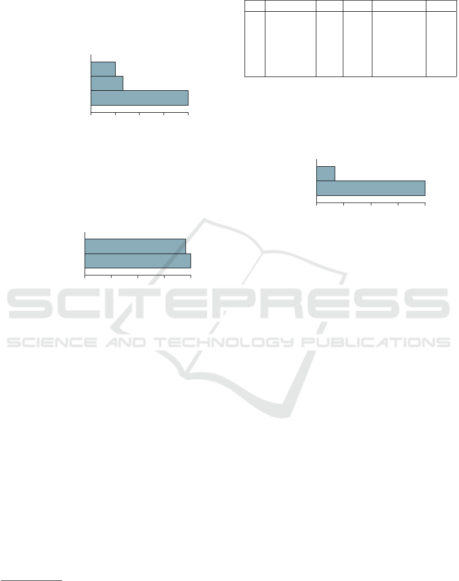
Compared with traditional compression methods
(ZIP), Figure 7 shows the relationship between the
original file, the compressed file with bit-to-bit and
the compressed file with the linux ZIP utility.
25%
7 bit by bit
33.3%
Float vector - zipped
100%
Float vector
0% 25% 50% 75% 100%
Figure 7: Compressed vector size.
Figure 8 shows the compression ratio between the
generated file with the bit-to-bit algorithm and the
same compressed file with the ZIP utility, as can be
seen, the compression ratio is very high, which shows
that the file generated with the proposed algorithm has
a high level of compression.
95.3%
7 bit by bit - zipped
100%
7 bit by bit
0% 25% 50% 75% 100%
Figure 8: Bit to bit vector size.
4.2 Public Dataset
In the case of public datasets, the compression method
was verified with the US Census Data (1990) Data Set
3
which contains 2458285 observations composed of
68 categorical attributes.
Table 3 shows the ranges of the 5 attributes with
the highest values. As it is observed, the iRemplpar
attribute has the biggest range [0,233], nevertheless it
has 16 categories. The compression used corresponds
to the number of categories of the attributes.
The iYearsch attribute has 18 categories. Accor-
ding to Section 3.2, the number of bits needed to
represent the values of each column corresponds to
Number o f bits = 5 with which it is possible to repre-
sent 6 elements per block.
The number of bytes required to store the data-
set without compression in memory
4
corresponds
to T b = (2458285 ∗ 68 ∗ 4) bytes = 668653520 bytes.
Thus, the amount of memory corresponds to T b =
637.68 Mbytes
5
.
3
https://archive.ics.uci.edu/ml/datasets/
US+Census+Data+(1990)
4
Most ML libraries requires integer values
5
R software shows 640 Mbytes of memory consumption
Table 3: US Census Data (1990) Data Set - Ranges.
N. Variable Min Max Max. value Cats.
1 iRemplpar 0 223 223 16
2 iRPOB 10 52 42 14
3 iYearsch 0 17 17 18
4 iFertil 0 13 13 14
5 iRelat1 0 13 13 14
... ... ... ... ... ...
The number of bytes needed to store the dataset
with compression in memory corresponds to: T bc =
(2458285 ∗ 68 ∗ 4)/6 bytes = 111442253,33 bytes
whereby the amount of memory corresponds to
T bc = 106.28 Mbytes. Figure 9 shows the compres-
sion ratio of the test dataset.
16.6%
Compressed
100%
Not compressed
0% 25% 50% 75% 100%
Figure 9: US Census Data (1990) Data Set - Memory con-
sumption.
5 CONCLUSIONS
In this document we reviewed some of the traditional
compression/encoding methods of categorical data.
In general, we can conclude that the proposal made
considerably reduce the amount of memory needed to
represent the data prior to be processed (see Figure 7).
The block decompression allows to process the data-
set without the need to completely decompress it prior
to the process, this allows to keep the dataset com-
pressed in memory instead of its uncompressed ver-
sion.
In the case of datasets with multiple columns, it
was shown that selecting the column with the most
categories provides a good compression ratio (see
Section 4.2). This can be optimized by taking into ac-
count the appropriate size for each column as it would
increase the compression ratio.
Future work may be proposed: (1) implement the
Basic Linear Algebra Subprograms (BLAS) standard
which defines low level routines to perform operati-
ons related to linear algebra which provide the ba-
sic infrastructure for the implementation of many ma-
chine learning algorithms and (2) implement com-
pression with larger block sizes (eg 64 bits).
Low Level Big Data Compression
357

ACKNOWLEDGEMENTS
The authors would like to thank to Universidad Cen-
tral del Ecuador and its initiatives Proyectos Semilla
and Programa de Doctorado en Informtica for the
support during the writing of this paper. This work
has been supported with Universidad Central del Ecu-
ador funds.
REFERENCES
Bruni, R. (2004). Discrete models for data imputation. Dis-
crete Applied Mathematics, 144(1-2):59–69.
Chen, Z., Gehrke, J., and Korn, F. (2001). Query optimiza-
tion in compressed database systems. ACM SIGMOD
Record, 30(2):271–282.
De Grande, P. (2016). El formato Redatam. ESTUDIOS
DEMOGR
´
AFICOS Y URBANOS, 31:811–832.
Elgohary, A., Boehm, M., Haas, P. J., Reiss, F. R., and
Reinwald, B. (2016). Compressed Linear Algebra for
Large-Scale Machine Learning. Vldb, 9(12):960–971.
Elgohary, A., Boehm, M., Haas, P. J., Reiss, F. R., and
Reinwald, B. (2017). Scaling Machine Learning via
Compressed Linear Algebra. ACM SIGMOD Record,
46(1):42–49.
Gan, G., Wu, J., and Yang, Z. (2009). A genetic fuzzy k-
Modes algorithm for clustering categorical data. Ex-
pert Systems with Applications, 36(2 PART 1):1615–
1620.
Hashem, I. A. T., Anuar, N. B., Gani, A., Yaqoob, I., Xia,
F., and Khan, S. U. (2016). MapReduce: Review and
open challenges. Scientometrics, 109(1):1–34.
Huang, Z. and Ng, M. K. (1999). A fuzzy k-modes algo-
rithm for clustering categorical data. IEEE Transacti-
ons on Fuzzy Systems, 7(4):446–452.
Ouyang, J., Luo, H., Wang, Z., Tian, J., Liu, C., and Sheng,
K. (2010). FPGA implementation of GZIP com-
pression and decompression for IDC services. Pro-
ceedings - 2010 International Conference on Field-
Programmable Technology, FPT’10, pages 265–268.
Rai, P. and Singh, S. (2010). A Survey of Clustering Techni-
ques. International Journal of Computer Applicati-
ons, 7(12):1–5.
Roman-gonzalez, A. (2012). Clasificacion de Datos Basado
en Compresion. Revista ECIPeru, 9(1):69–74.
Seshadri, V., Hsieh, K., Boroumand, A., Lee, D., Kozuch,
M. A., Mutlu, O., Gibbons, P. B., and Mowry, T. C.
(2015). Fast Bulk Bitwise and and or in DRAM. IEEE
Computer Architecture Letters, 14(2):127–131.
KDIR 2018 - 10th International Conference on Knowledge Discovery and Information Retrieval
358