
Multi-objective Evolutionary Approach in the Linear Dynamical
System Inverse Modeling
Ivan Ryzhikov
1,2
, Christina Brester
1,2
, Eugene Semenkin
2
and Mikko Kolehmainen
1
1
Department of Environmental and Biological Sciences, University of Eastern Finland, Kuopio, Finland
2
Institute of Computer Science and Telecommunications, Reshetnev Siberian State University of Science and Technology,
Krasnoyarsk, Russia
Keywords: Time-invariant System, Dynamical System, Linear Differential Equation, Inverse Problem, Multi-objective
Optimization, System Identification, Initial Value.
Abstract: In this study, we consider an inverse mathematical modeling problem for dynamical systems with a single
output. Generally, the final solution of this problem is an approximation of a system transient process and a
system state at some time point. Only those classes of models, which describe the transient process properly,
can portray the system behavior and can be applicable for prediction and optimal control problems. One of
possible mathematical representations of dynamical systems is differential equations, in particular, linear
differential equations for linear systems. While solving the inverse problem, we aim to identify a differential
equation order and parameters, an initial system state. Since all the parameters are interrelated, we propose
to identify them by solving a two-criterion optimization problem, which includes the model adequacy (i.e. a
distance between model outputs and observations) and the closeness of the initial value estimation to the
observation data. To solve this complex optimization problem, we apply a Real-valued Cooperative Multi-
Objective Evolutionary Algorithm which effectiveness has been proved on the set of high-dimensional test
problems. We investigate the dependency between the considered criteria by depicting the Pareto front
approximation. Then, having the same amount of computational resources, we vary the system order, the
number of control inputs and the initial state to analyze changes in the algorithm effectiveness based on
each criterion and estimate basic limitations. Finally, we conclude that the optimization problem considered
is quite challenging and it might be used for testing and comparing various heuristics.
1 INTRODUCTION
Inverse mathematical modeling problems of
dynamical systems occur in different scientific and
practical fields. In most cases, identification
approaches are applicable only for processes and
systems for which the transient processes and the
initial state are known or there are some acceptable
assumptions about them. Basically, one needs to
approximate the system parameters so that the model
output would fit the observation data in the best
way. However, when we solve the identification
problem in a general case, there is no information
about the following things: the mathematical
operator class of the transient process, mathematical
model parameters and the initial system state.
Moreover, all these variables have a complex
influence on the model adequacy.
In this study, we consider the inverse modeling
problem reduction to a two-criterion optimization
problem. The reduced problem includes the
following criteria: the first one reflects the distance
between the observation data and the model output
and the other one means the distance between the
initial value estimation and the data at the beginning
of the process observation. This multi-objective
problem formulation exposes the relation between
the transient process and the initial system state. The
main idea behind this two-objective problem is that
different initial system states can produce different
optimization problems for parameters and vice-
versa. Therefore, the system initial state and the
transient process must be approximated
simultaneously (Ryzhikov et al., 2016).
The approximation of the transient process
differs from the standard regression problem
because the identification is applied to the field of
differential operators and the system input is not the
element of the vector field, but the piecewise
continuous function. In this study, we assume that
Ryzhikov, I., Brester, C., Semenkin, E. and Kolehmainen, M.
Multi-objective Evolutionary Approach in the Linear Dynamical System Inverse Modeling.
DOI: 10.5220/0007228402810288
In Proceedings of the 10th International Joint Conference on Computational Intelligence (IJCCI 2018), pages 281-288
ISBN: 978-989-758-327-8
Copyright © 2018 by SCITEPRESS – Science and Technology Publications, Lda. All rights reserved
281

the dynamical system can be described with the
linear differential equation. Thus, the inverse
modeling problem can be reduced to the
identification of the differential equation order, its
parameters and the initial state vector. In previous
studies, such as (Ryzhikov et al., 2016) and
(Ryzhikov and Semenkin, 2017), we have
considered one-criterion approaches. We discovered
that solving this problem requires some specific and
problem-oriented algorithm modifications.
Nevertheless, these studies lack thorough
experiments for systems with different orders, the
number of control inputs and different initial states.
To solve the two-criterion optimization problem,
we use a Real-valued Multi-Objective Evolutionary
Algorithm based on the island model cooperation,
which includes the following heuristics as the
parallel working islands: the Strength Pareto
Evolutionary Algorithm (SPEA2) (Zitzler et al.,
2002), the Preference-Inspired Co-Evolutionary
Algorithm with goal vectors (PICEA-g) (Wang,
2013), and the Non-dominating Sorting Genetic
Algorithm II (NSGA-II) (Deb et al., 2002).
Previously, the proposed algorithm with the binary
solution representation was successfully applied for
solving different optimization problems (Brester and
Semenkin, 2015) and particular inverse modeling
problems (Brester et al., 2016a), (Semenkina et al.,
2014) and (Brester et al., 2016b).
In the study (Ryzhikov et al., 2017), the inverse
modeling problem for chemical disintegration
reaction was reduced to the multi-criteria
optimization problem, which was solved with the
cooperation of the multi-objective evolutionary
algorithms. That considered approach achieved the
promising results and allowed us to solve the general
inverse problem for the linear dynamical system.
Our goal is to explore the algorithm performance for
this problem and estimate how its efficiency changes
when varying the initial problem parameters: the
system order, the number of control inputs and the
initial state vector. This is needed to reveal when
and how the complexity changes.
2 INVERSE MATHEMATICAL
MODELING PROBLEM FOR
LINEAR DYNAMICAL
SYSTEMS
Let us consider a linear time-invariant system
inverse modeling problem. It is assumed that the
initial system can be determined with a linear
differential equation (LDE)
()
01
nm
i
i j j
ij
a x t b u t
,
(1)
where
()
: , 0,
i
x t i n
is the system state i-
th derivative,
: , 1,
j
u t j m
is the j-th
input function, n and m are the differential equation
order and the number of input functions,
respectively. Here, with the notation
(0)
xt
we
mean the function
xt
itself.
Using the equation (1), we can evaluate the
model output on some particular set of inputs if we
know the system state at the initial time
0
t
. Let us
denote the system state as
n
v
, so
0
x t v
and
that would lead us to the following Cauchy problem
()
01
nm
i
i j j
ij
a x t b u t
,
0
x t v
.
(2)
Now let the sets
, , 1,
ii
Y y T t i s
be an
observation data, where
i
y
are the system
output measurements at times
i
t
, and
s
is the
number of observations. It is assumed, that the
system output and the observations can be
determined with the following equation
( ) , 1,
i i i
y x t i s
,
(3)
where
: ( ) 0, ( )ED
is a random value and
()
i
xt
is the solution of the Cauchy problem (2) at
the time point
i
tt
.
In this study, we assume that the order of the
differential equation (1) is given. Thus, we need to
identify the parameters of the differential equation
(1) and the initial value of the related Cauchy
problem (2). In other words, the problem can be
reduced to determine the parameters and initial
values, which would maximize fitting the
observation data by the solution of the Cauchy
problem
1
( ) ( )
01
ˆ
ˆ
nm
ni
i j j
ij
x t a x t b u t
,
0
ˆ
x t v
,
0
mintT
,
(4)
where
ˆ
n
a
,
ˆ
m
j
b
and
ˆ
n
v
. The Cauchy
problem (4) is modified, because if we know the
LDE order, then its first coefficient cannot be equal
to 0 and, thus, the equation (2) can be transformed to
the equation (4), by dividing all its coefficients by
this coefficient.
According to the model representation (4) and
using the observation data
Y
and
T
, the inverse
IJCCI 2018 - 10th International Joint Conference on Computational Intelligence
282

modeling problem can be reduced to the two-
criterion optimization problem with the following
criteria:
1
1
1
ˆ
ˆˆ
,,
min
s
ii
i
a b v
y x t
C
s
,
(5)
2
argmin
ˆ
1
min min
i
T
v
C y x T
.
(6)
The first criterion (5) is a standard one that
estimates the model adequacy. The second criterion
(6) is the measure of the closeness of the initial
value estimation to the observation data set. In this
study, the norm of each criterion is chosen as the
Manhattan norm. The reason for this decision is its
better robustness against the abnormal values.
As one can see, the LDE coefficients have no
influence on the second criterion, but the initial
value estimation influences the main criterion (5).
The solution of the problem considered is the
Pareto set of non-dominated alternatives. The Pareto
set can be determined as
22
::
n m n m
P p z z p
, where
with the notation
12
zz
we mean that both
1 1 1 2
С z С z
and
2 1 2 2
С z С z
conditions
are met and at least one of the following conditions
is met:
1 1 1 2
С z С z
or
2 1 2 2
С z С z
. It is
impossible to calculate the Pareto set analytically, as
well as, the Pareto front for the problem (5)-(6), and,
thus, we need to approximate it.
The solution of the Cauchy problem (4) is
evaluated with the Runge-Kutta 4-th order numerical
integration scheme. For each particular considered
Cauchy problem, the initial and final integration
time points are known and the integration step is
equal to 0.05.
All the identification problems considered in this
study have been generated without the additive
noise. We can consider the performance of the
modeling approach, regardless the distortion of the
observation data.
3 MULTI-OBJECTIVE
COOPERATIVE GENETIC
ALGORITHM WITH THE
ISLAND META-HEURISTIC
In multi-objective optimization, we aim at achieving
a compromise between competing criteria. The
Pareto-dominance idea (Goldberg, 1989) is widely
used to compare alternative solutions. While solving
multi-criteria problems, we expect to obtain a set of
non-dominated points, which cannot be preferred to
one another based on all the objectives considered.
Evolutionary-based algorithms (in particular,
Genetic Algorithms (GAs)) operate with a set of
solutions at each generation, and therefore, they
were considered as an effective tool to find Pareto
set and front approximations. Nevertheless, there are
some open questions researchers usually face when
they apply Multi-Objective Evolutionary Algorithms
(MOEAs) in practical problems.
Firstly, different fitness assignment strategies
might be proposed (Zitzler, 2004): the dominance
depth, the dominance rank or the dominance count
might be used to assign a fitness function.
Next, various diversity preservation techniques
might be applied. In (Silverman, 1986) these
techniques are introduced: nearest neighbour
techniques, kernel methods, histograms.
Furthermore, the idea of elitism has been
proposed to avoid the loss of good individuals
during the stochastic algorithm execution. There are
two ways to implement it: to merge the parent
population with the offspring and then to employ
environmental selection or to use an additional set
for keeping promising solutions.
Remembering these issues, we decided to apply a
cooperative MOEA (Brester and Semenkin, 2015)
which includes three algorithms based on different
heuristics. The cooperative MOEA enables us to
eliminate the choice of the appropriate algorithm and
avoid many experiments with different MOEAs. The
cooperative MOEA uses an island model (Whitley et
al., 1997) and includes NSGA-II, PICEA-g, and
SPEA2 as its islands work in a parallel way. The
initial number of individuals is spread across
subpopulations equally. The fitness function
evaluation for different subpopulations is
implemented in parallel threads. At each T-th
generation algorithms exchange the best solutions
(migration). There are two parameters: migration
size, the number of candidates for migration, and
migration interval, the number of generations
between migrations.
Moreover, the island model topology should be
determined, in other words, the scheme of migration.
The fully connected topology is applied, meaning
that each algorithm shares its best solutions with all
other algorithms included in the island model.
Originally, GAs operate with binary strings,
however, for real-valued optimization problems a
number of genetic operators have been developed.
Multi-objective Evolutionary Approach in the Linear Dynamical System Inverse Modeling
283

To select effective solutions for the offspring
generation, we apply binary tournament selection.
As a crossover operator, we use intermediate
recombination. In a mutation operator, we
implement the next scheme (Liu et al., 2009):
,,
( ), ,
'
m
m
j j j j
j
j
Up
Up
x b a
x
x
(7)
With
1
1
1
1
(2 ) 1, if 0.5
1 (2 2 ) , otherwise
j
rand U
rand
(8)
where U is a uniformly random number [0, 1]. There
are two control parameters: the mutation rate
n
p
m
1
, where n is the chromosome length, and the
distribution index
is equal to 1.0.
j
a
and
j
b
are
the lower and the upper bounds of the j-th variable
in the chromosome.
The cooperative MOEA was investigated on the
set of complex benchmark problems CEC 2009
(Zhang, 2008) and proved its effectiveness (Brester
and Semenkin, 2015).
4 INVERSE MODELING
PROBLEM SOLVING
In the experiments conducted, we considered
different LDEs and Cauchy problems: we varied the
order of the LDE, the initial values and the number
of the inputs. To solve all the considered problems,
the proposed MOEA was applied. The maximum
number of objective function evaluations was 30000
for each algorithm in the island model. Each
algorithm had 300 generations and 100 individuals
for its population. The migration interval was 25
generations and the migration set size was 10. The
limitation of the total amount of the fitness function
evaluations was 90000. For each problem, the
MOEA was launched for 20 times.
The initial population was generated randomly
within the hypercube
2
1,1
nm
, and the borders for
the heuristic search were
2
5, 20
nm
. The
influence of the initial population generation on the
algorithm efficiency is beyond the scope of this
article.
First, we analyzed the influence of the LDE
order. The coefficients of the LDE are given in
Table 1. The input function for these experiments
was chosen as the unit-step function,
,1u t t m
. The initial values of the system
and the coefficients of the control inputs were equal
to
0
d
R
and 1, respectively, and
d
was the LDE
order. The fixed control coefficients and initial
values allowed us to estimate the complexity
growth, which was caused only by the order
increase. The initial time was equal to 0 for all the
Cauchy problems. The final time was equal to 10 for
problems of orders 2 or 3 and 20 for problems of
other orders.
Table 1: Cauchy problems: orders and equation
coefficients.
Order
Parameters
2
1, 2a
3
1, 2,1a
4
1, 2, 4,1a
5
0.25,1.75, 4.75, 6.25, 4a
6
0.25, 2,6.5,11,10.25,5a
7
0.125,1.25, 5.25,12,16.125,12.75, 5.5a
The results obtained are given in Figures 1 and 2
for the first criterion (5) and the second one (6),
respectively, and boxplots reflect the algorithm
efficiency. The best solution, according to each
criterion, was chosen from the Pareto front
estimation in each particular algorithm run. We can
see that the first criterion (5) values become worse
with the increase of the LDE order and this
deterioration is nonlinear. The second criterion (6)
values are close to 0, which is not informative, in
contrast to the first one, therefore, we exclude it
from the further analysis and focus on the Pareto
front estimations and the first criterion (5)
distribution.
Figure 1: Pareto front estimation statistics for different
LDE orders. The first criterion (5).
IJCCI 2018 - 10th International Joint Conference on Computational Intelligence
284
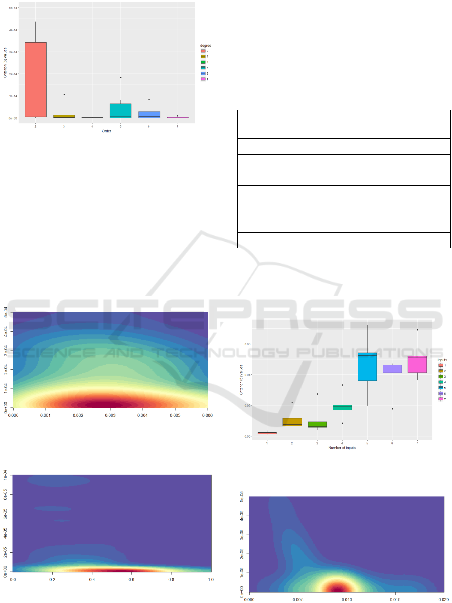
Figure 2: Pareto front estimation statistics for different
LDE orders. The second criterion (6).
In Figures 3 and 4, the Pareto front estimation
distributions are presented for the system of the 2nd
order and for the system of the 7th order,
respectively.
The heat maps show that the distribution of the
solutions for the system of the 7
th
order is more
complex. For the 2
nd
order systems the distribution
of the front approximation is closer to 0 by the first
criterion (5). At the same time, for the 7
th
order the
distribution is much closer to 0 by the second
criterion (6).
Figure 3: The Pareto front distribution for the 2
nd
order
inverse problem (Table 1). X-axis corresponds to the first
criterion, Y-axis corresponds to the second criterion.
Figure 4: The Pareto front distribution for the 7
th
order
inverse problem (Table 1). X-axis corresponds to the first
criterion, Y-axis corresponds to the second criterion.
The next factor is the number of control inputs
and their influence on the problem complexity. To
investigate it, we performed the same experiment for
the system of the 2
nd
order from Table 1, for which
the control inputs are listed in Table 2. The initial
values were equal to 0 and the final integration time
was 10.
Table 2: Cauchy problems: control inputs.
Number of
inputs,
m
Input:
1
m
j
j
ut
1
1
u t t
2
2
sinu t t
3
3
cosu t t
4
4
u t t
5
5
sin 2u t t
6
6
cos 2u t t
7
7
ln 1u t t
The results of the Pareto front estimation for
problems with different number of inputs are given
in Figure 5. The distributions of the Pareto front for
one and seven control inputs are given in Figures 6
and 7, respectively.
Figure 5: Pareto front estimation statistics for the different
number of inputs. The first criterion (5).
Figure 6: The Pareto front distribution for the 2
nd
order
inverse problem (Table 1) and one control input (Table 2).
Multi-objective Evolutionary Approach in the Linear Dynamical System Inverse Modeling
285
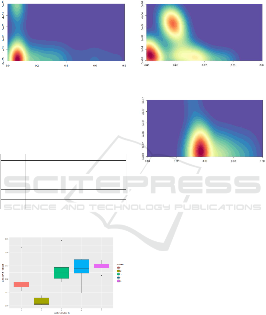
Figure 7: The Pareto front distribution for the 2
nd
order
inverse problem (Table 1) and seven control inputs (Table
2).
Then, we considered the initial value of the
system and its influence on the problem complexity.
For this experiment, we took the system of the 4
th
order from Table 1. The different initial values are
given in Table 3. The final integration time was
equal to 15 and the input was the unit-step function.
Table 3: Cauchy problems: initial values.
Problem
Initial value
1
0000v
2
1 0 0 0v
3
0 1 0 0v
4
0 0 1 0v
5
0 0 0 1v
The results of the Pareto front estimations for the
different combinations of the initial values are given
in Figures 8, 9 and 10.
Figure 8: Pareto front estimation statistics for different
initial values (Table 3). The first criterion (5).
All the Cauchy problems were considered for the
stable LDEs. Here the stable system was generated
via the characteristic equation so that each root had
the negative real part.
Figure 9: The Pareto front distribution for the 4
th
order
inverse problem (Table 1) and the 2
nd
initial value (Table
3).
Figure 10: The Pareto front distribution for the 2
th
order
inverse problem (Table 1) and the 5
th
initial value (Table
3).
As the Pareto front distribution approximations
show, the front is localized but still has a complex
structure. Anyway, the inverse mapping of the close
Pareto front elements could give us completely
different alternatives, which makes the inverse
modeling problem complex.
5 CONCLUSION
In this study, the inverse mathematical modeling
problem was reduced to the two-criterion
optimization problem on the real vector space,
which was solved by the real-valued cooperative
MOEA.
The complexity of the problem considered
depends on the LDE order, the number of inputs and
the initial values. The complexity growth can be
estimated by changing the objective criterion values,
which are found by the MOEA. In our experiments,
the computational resources were the same for all
the problems, so it was possible to estimate the
influence of the certain parameter, such as the
differential equation order, the number of inputs and
the initial state.
IJCCI 2018 - 10th International Joint Conference on Computational Intelligence
286

The order of the differential equation has the
strongest effect on the algorithm efficiency and thus,
the problem complexity. The possible reason for that
is not only the increased dimension of the search
space, but also the increased variance and the
maximum absolute value of the LDE coefficients,
which makes the search space wider. The increase of
the order by 1 increases the dimension by 2, since
each order is related to the coefficient and the initial
value.
The number of control inputs also determines the
search space dimension and makes the reduced
problem more complex, when the number of inputs
increases. There is another significant detail, which
is hard to be formalized: when the number of inputs
increases, their impacts overlap and this can mislead
the algorithm.
The search space dimension does not change
when we vary the initial values. However, the
problem becomes more challenging, as there are the
initial values of the high orders, which are not equal
to 0. Therefore, changing the analyzed parameters,
we may create various challenging test problems for
MOEAs.
Future research will be related to the estimation
of the computational resources, which would be
required to keep the algorithm performance at the
same level while changing the parameters. This
study is a prior to the development of the automatic
identification of the causative control inputs and the
differential equation order. The gathered information
also would be used to develop the problem-oriented
algorithms with higher performance.
ACKNOWLEDGEMENTS
The reported research was funded by Russian
Foundation for Basic Research and the government
of the region of the Russian Federation, grant № 18-
41-243007.
REFERENCES
Brester, C., Kauhanen, J., Tuomainen, T.P., Semenkin, E.,
Kolehmainen, M., 2016. A. Comparison of two-
criterion evolutionary filtering techniques in
cardiovascular predictive modelling. Proceedings of
the 13th International Conference on Informatics in
Control, Automation and Robotics (ICINCO’2016),
Lisbon, Portugal, vol. 1: pp. 140–145.
Brester, C., Semenkin, E., 2015. Cooperative
Multiobjective Genetic Algorithm with Parallel
Implementation. Advances in Swarm and
Computational Intelligence, LNCS 9140: pp. 471–
478.
Brester, C., Semenkin, E., Sidorov, M., 2016. B. Multi-
objective heuristic feature selection for speech-based
multilingual emotion recognition. Journal of Artificial
Intelligence and Soft Computing Research, vol. 6, no.
4: pp. 243-253.
Deb, K., Pratap, A., Agarwal, S., Meyarivan, T., 2002. A
fast and elitist multiobjective genetic algorithm:
NSGA-II. IEEE Transactions on Evolutionary
Computation 6 (2): pp. 182-197.
Goldberg, D., 1989. Genetic algorithms in search,
optimization, and machine learning. Addison-wesley.
Liu, M., Zou, X., Chen, Y., Wu, Z., 2009. Performance
assessment of DMOEA-DD with CEC 2009 MOEA
competition test instances. 2009 IEEE Congress on
Evolutionary Computation.
Ryzhikov, I., Semenkin, E., 2017. Restart Operator Meta-
heuristics for a Problem-Oriented Evolutionary
Strategies Algorithm in Inverse Mathematical MISO
Modelling Problem Solving. IOP Conference Series:
Materials Science and Engineering, vol. 173.
Ryzhikov, I., Semenkin, E., Panfilov, I., 2016.
Evolutionary Optimization Algorithms for Differential
Equation Parameters, Initial Value and Order
Identification. ICINCO (1) 2016: pp. 168-176.
Ryzhikov I., Brester Ch., Semenkin E. Multi-objective
dynamical system parameters and initial value
identification approach in chemical disintegration
reaction modelling. Proceedings of the 14th
International Conference on Informatics in Control,
Automation and Robotics (ICINCO’2017), Madrid,
Spain, vol. 1: pp. 497-504.
Semenkina, M., Akhmedova, Sh., Brester, C., Semenkin,
E., 2016. Choice of spacecraft control contour variant
with self-configuring stochastic algorithms of multi-
criteria optimization. Proceedings of the 13th
International Conference on Informatics in Control,
Automation and Robotics (ICINCO’2016), Lisbon,
Portugal, vol. 1: pp. 281–286.
Silverman, B., 1986. Density estimation for statistics and
data analysis. Chapman and Hall, London.
Wang, R., 2013. Preference-Inspired Co-evolutionary
Algorithms. A thesis submitted in partial fulfillment
for the degree of the Doctor of Philosophy, University
of Sheffield: p. 231.
Whitley, D., Rana, S., and Heckendorn, R., 1997. Island
model genetic algorithms and linearly separable
problems. Proceedings of AISB Workshop on
Evolutionary Computation, vol.1305 of LNCS: pp.
109-125.
Zhang, Q., Zhou, A., Zhao, S., Suganthan, P. N., Liu, W.,
Tiwari, S., 2008. Multi-objective optimization test
instances for the CEC 2009 special session and
competition. University of Essex and Nanyang
Technological University, Tech. Rep. CES–487, 2008.
Zitzler, E., Laumanns, M., Bleuler, S., 2004. A Tutorial on
Evolutionary Multiobjective Optimization. In:
Gandibleux X., (eds.): Metaheuristics for
Multi-objective Evolutionary Approach in the Linear Dynamical System Inverse Modeling
287

Multiobjective Optimisation. Lecture Notes in
Economics and Mathematical Systems, Vol. 535,
Springer.
Zitzler, E., Laumanns, M., Thiele, L., 2002. SPEA2:
Improving the Strength Pareto Evolutionary Algorithm
for Multiobjective Optimization. Evolutionary
Methods for Design Optimisation and Control with
Application to Industrial Problems EUROGEN 2001
3242 (103): pp. 95-100.
IJCCI 2018 - 10th International Joint Conference on Computational Intelligence
288
