Circulating Tumor Enumeration using Deep Learning

Stephen Obonyo and Joseph Orero

Faculty of Information Technology, Strathmore University, Ole Sangale Link Road, Nairobi, Kenya

Keywords:

CTC Enumeration, CTC Detection, Artiﬁcial Neural Networks, Machine Learning, Deep Learning.

Abstract:

Cancer is the third most killer disease just after infectious and cardiovascular diseases. Existing cancer treat-

ment methods vary among patients based on the type and stage of tumor development. Treatment modalities

such as chemotherapy, surgery and radiation are successful when the disease is detected early and regularly

monitored. Enumeration and detection of Circulating Tumor Cells (CTC’s) is a key monitoring method which

involves identiﬁcation of cancer related substances known as tumor markers which are excreted by primary

tumors into patient’s blood. The presence, absence or number of CTC’s in blood can be used as treatment

metric indicator. As such, the metric can be used to evaluate patient’s disease progression and determine ef-

fectiveness of a treatment option a patient is subjected to. In this paper, we present a deep learning model

based on Convolutional Neural Network which learns and enumerates CTC’s from stained image samples.

With no human intervention, the model learns the best set of representations to enumerate CTC’s.

1 INTRODUCTION

Cancer is a disease occurring as a result of genetic

mutation or abnormal changes in the genes responsi-

ble for regulating the growth of body cells. The cells

gain ability to keep dividing without control, produ-

cing more cells and forming a tumor (Ferlay et al.,

2010). The abnormal cells inﬁltrates healthy ones and

spreads throughout the body.

According to Fitzmaurice et al. (2015) cancer cau-

sed more than 8 million deaths globally in the year

2013. The cancer death burden have been recorded in

both ﬁrst and third world countries though in an une-

qual measure. Cancer cases have been exacerbated by

unique geographical, cultural and demographic fac-

tors such as aging population and increased predispo-

sition to cancer causing conditions such as smoking,

being overweight and physical inactivity.

The death ﬁgures in ﬁrst world countries are re-

latively lower as compared to third world countries.

Developing nations have contributed to 57% of can-

cer total cases. This percentage accounts for approxi-

mately 65% of related deaths worldwide (Torre et al.,

2015). The higher ﬁgures can be attributed to inabi-

lity to access proper medication and lack of regular

monitoring.

Today, different types of cancer are treatable if de-

tected early. Standard medical detection modalities

include Radiography, Magnetic Resonance Imaging

(MRI), Computer Tomography (CT) and Ultrasound.

After cancer detection process, a patient is subjected

to appropriate treatment option based on stage and

type of tumor. For a given patient, medical surgery or

radiation would apply, for others chemotherapy, while

hormone therapy for other subjects.

During treatment, a patient must be constantly

monitored to determine effectiveness of treatment

method they are subjected to. This can be achieved

through medical processes such as biopsy or liquid

biopsy. Biopsy is a medical procedure which can be

used to detect tumor related substances known as Ci-

rculating Tumor Cells (CTC’s). The process involves

identiﬁcation of CTC’s in a raw body tissues. In con-

trast, liquid biopsy involves detection of the CTC’s in

blood after staining the sample.

Tumors excretes CTC’s into patient’s blood. Du-

ring treatment, the presence, absence or the number

CTC’s in blood can be used as patient’s progress me-

tric indicator to evaluate how the subject is responding

to treatment. The metric also determines the effecti-

venesses of treatment option one is enrolled in. Besi-

des monitoring cancer treatment response and deter-

mining the effectiveness of a treatment method, biop-

sies are also key in assessing the cancer recurrence

and progression (Crowley et al., 2013).

In this research work, we present a CTC enumera-

tion model. We show how Convolutional Neural Net-

work (ConvNet) can be used to learn intricate featu-

res for enumerating CTC’s in a given stained sample

image.

Obonyo, S. and Orero, J.

Circulating Tumor Enumeration using Deep Learning.

In Proceedings of the 10th International Joint Conference on Computational Intelligence (IJCCI 2018), pages 297-303

ISBN: 978-989-758-327-8

297

An image sample may contain more than one CTC

or none. Based on this, we developed an algorithm

to locate CTC’s and generate training samples from

an input image. We also show that certain models are

incapable of learning abstract representative details as

opposed to the preferred model.

2 RELATED WORK

Application of learning models in cancer manage-

ment have been presented by many researchers. Sim-

ple and classical learning approaches such as decision

trees have been used in detection of common Circula-

ting Tumors variations such as Cytokeratin, Apoptic

and Debris. CTC’s are extracted following standard

procedures such as ﬁctionalized and structured medi-

cal wire, Epithelial Cell Adhesion Molecule, density

gradient centrifugation or membrane ﬁltration. Schol-

tens et al. (2012) used Random Forests and Decision

Trees to classify CTC’s. The target labels were based

on different CTC classes such as Apoptic CTC, CTC

debris, Leukocytes and Debris.

In another study, Svensson et al. (2014) presen-

ted how Naive Bayes classiﬁer and Generative Mix-

ture Model can be used to detect CTC’s in stained

blood sample. Cells were collected using ﬁctionali-

zed medical wire and thereafter stained. The intensity

of RGB (Red, Green, Blue) values of the resulting

sample was then used as the input features to the mo-

del. The classiﬁer learned to discriminate an instance

given the predeﬁned CTC’s class.

Aside from classical learning approaches such as

Decision Trees, Naive Bayes among other algorithms,

deep learning models have also been applied. This le-

arning methodology have led to much better results

in image detection and recognition. According to Le-

Cun et al. (2015) deep learning methods have impro-

ved the state-of-the-art visual object recognition and

detection. This learning approach can automatically

discover best set of features to represent an instance.

This unique characterization has contributed to unpre-

cedented success studies in the ﬁeld of image recog-

nition.

Mao et al. (2016) proposed use of Deep Convo-

lutional Neural Network, a deep learning model, to

detect Circulating Tumor Cells. The model automati-

cally learned the best set of features used to classify a

sample as either having CTC or not. They demonstra-

ted that automated feature discovery using the lear-

ning model led to much better results than hand craf-

ted. There was a signiﬁcant variation in performance

when their proposed model was compared to the clas-

sical ones such as Support Vector Machines with ma-

nually engineered input features.

Wang et al. (2016) also employed a similar lear-

ning technique in detection of tumor recurrence yiel-

ding state of the art results. In the work, deep learning

model developed was aimed at predicting the extent

of cancer spread to the other parts of the body.

3 METHODOLOGY

3.1 Dataset

Data used in this research work was secondary data.

It was provided by a PhD candidate in Computer

Science from Missouri University of Science and

Technology. It is the same dataset used in (Mao et al.,

2016). The original work was based on classiﬁcation

of CTC’s as opposed to enumeration which this pa-

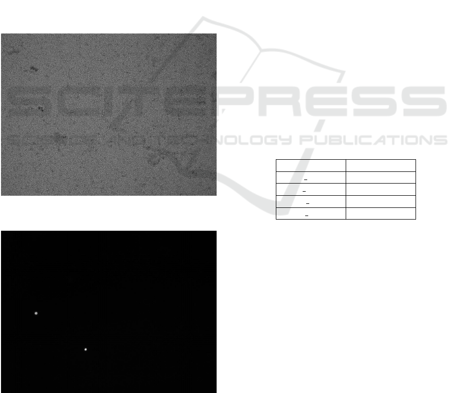
per focuses on. Figure 1 and Figure 2 shows sample

images. Figure 1 is a sample of microscopy image.

Figure 2 on the other hand is a sample ﬂuorescence

image. The latter is used to locate the exact loca-

tion of the CTC’s in the former. Every microscopy

image has a corresponding ﬂuorescence image sho-

wing CTC’s locations.

We developed an algorithm to extract the regions

of interest (ROI) to generate both the positive (with

CTC) and negative (without CTC) training and testing

sets. A total of 1904 training samples were generated.

Out of this, 952 were positive and 952 negative. Every

sample had a corresponding target label equivalent to

the number of CTC’s contained. Positive samples had

N CTC’s and 0 for negative instances. 80% of the

dataset was used for training and the remaining 20%

for testing the model.

3.2 Cropping Algorithm

We developed an algorithm to extract 40 by 40 the

regions of interest (ROI). It accepts x and y coordi-

nates of CTC location in the ﬂuorescence image and

a corresponding microscopy image. Following this,

20-pixel coordinate location to the left of x and to the

right are marked and saved. The same process also

applies for the y coordinate. Random x coordinate

within image width range is generated and another

random y within image height range. These random x,

y values represent the location of new negative sam-

ple instance. If these randomly generated coordinates

range do not overlap with CTC location bounds then

positive and negative sample is cropped out from the

1600x1600 input image and returned. The algorithm

have been summarized by Listing 1.

IJCCI 2018 - 10th International Joint Conference on Computational Intelligence

298

crop_sample(xpixel, ypixel, image)

counter <- 1

initialise xaxes[], yaxes[]

initialise samples[]

xaxes[0] <- xpixel

yaxes[0] <- ypixel

for left_coordinates and

right_coordinates do:

while counter < 21

xaxes[counter+1] = xpixel + counter

yaxes[counter+1] = ypixel + counter

counter <- counter+1

randomx <- random{0,1580}

randomy <- random{0,1280}

if x intersection xaxes is empty and

y intersection yaxes is empty

samples[0] <- crop(xpixel,ypixel)

samples[1] <- crop(x,y)

return samples

Listing 1: The Cropping Algorithm.

Figure 1: 1600x1600 A microscopy image containing

CTC’s.

Figure 2: 1600x1600 Fluorescence image depicting loca-

tion of CTC’s in Figure 1.

3.3 Training Set Generation

Microscopy images contains CTC’s within speciﬁc

locations. These images were all converted to one

channel from RGB. Fluorescence images on the other

hand shows the location or coordinates of CTC’s. All

images in this set were converted to gray scale and bi-

nary thresholded. Thresholding helped to accurately

locate the Circulating Tumors Cells.

Binary thresholding involves converting all the

image pixels to either of the two predeﬁned values;

black or white (Gonzalez and Woods, 2002). To

achieve this, pixel intensity values less than 240 were

set to 0 and 255 otherwise for the ﬂorescence images.

All ﬂuorescence image samples were thresholded

using similar function and x, y coordinates of white

pixels then mapped to the corresponding one channel

microscopy image. This process was then followed

by cropping out a positive and negative samples of

dimension 40 by 40. The negative set was generated

by randomly generating x, y coordinates, checking for

the overlap with the positive sample bounds and crop-

ping then cropping out. The feature set was created in

this fashion repeating the process over all the images.

The target labels for the negative samples were set 0

and N; number of white pixels for the positive instan-

ces. Resulting feature sets and targets were persis-

tently stored. Table 1 summarizes the dimensions of

training and testing dataset dimensions. Cropped po-

Table 1: A summary of training and testing dataset dimen-

sions.

Dataset Dimension

X train (1523, 40, 40)

y train (1523, 1)

X test (381, 40, 40)

y test (381, 1)

sitive and negative samples exhibit different patterns.

A high-level depiction of this variation is illustrated

by Figure 3 and Figure 4. Figure 3 shows sample posi-

tive while Figure 4 represents negative both randomly

sampled from training dataset.

3.4 Model Architecture

Convolutional Neural Network (ConvNet) model was

used to enumerate the CTC’s given the feature sets

and labels. The model architecture is captured by Fi-

gure 5. The network predicts number of CTC’s given

an image sample thus a regression task. The ConvNet

is composed of Convolution - Max Pooling - Convo-

lution - Max Pooling - Fully Connected Layer (FC1)

- Fully Connected Layer (FC2). The architecture is

shown by Figure 5 During forward propagation 40 by

Circulating Tumor Enumeration using Deep Learning

299

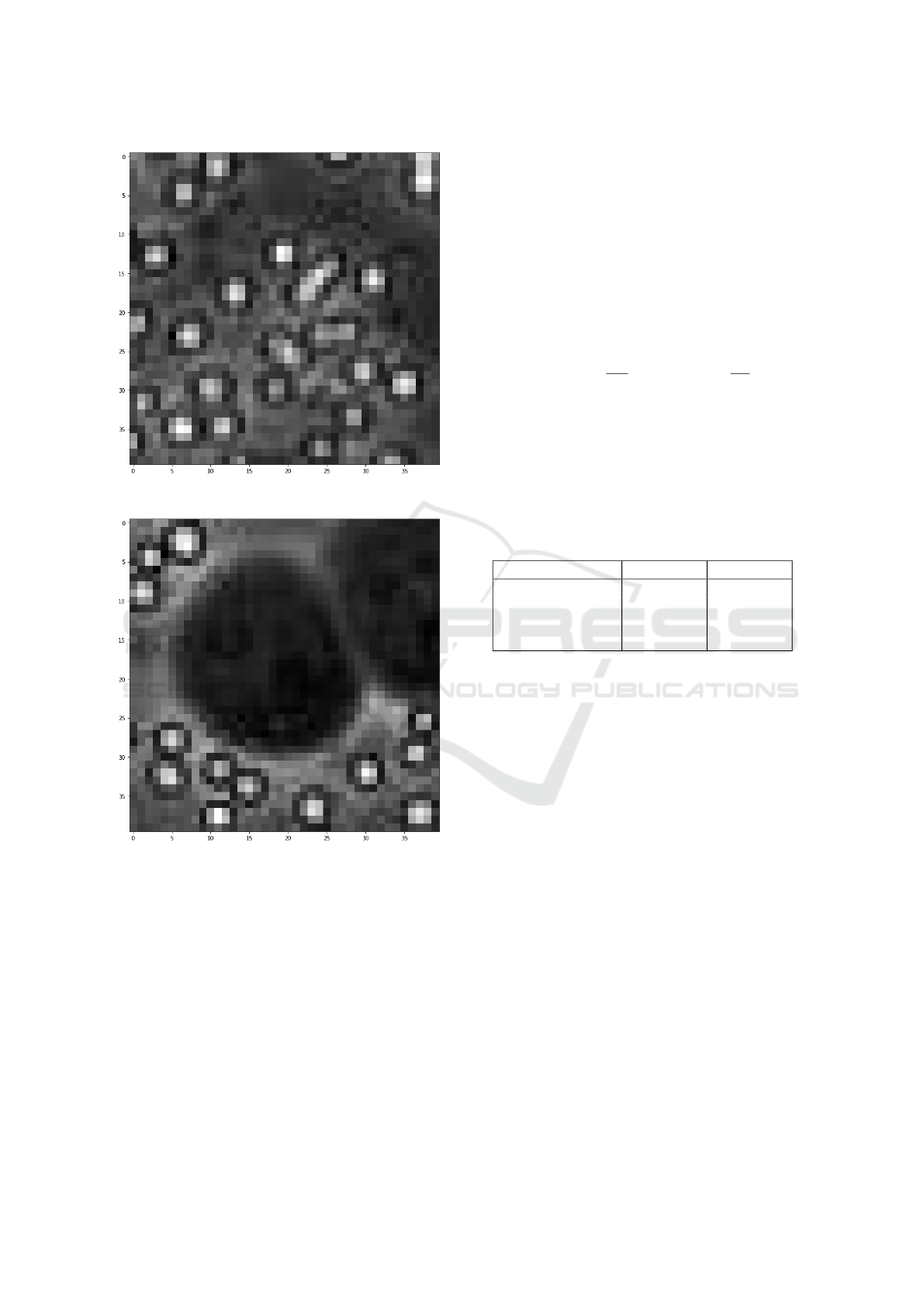
Figure 3: Cropped 40x40 negative sample with 0 CTC’s.

Figure 4: Cropped 40x40 positive sample with given num-

ber of CTC’s.

40 input was fed into the network. A kernel of shape

5*5 was used to convolve the input image with a slide

of 1 resulting in 8 feature maps. The convolution step

was then followed by Rectiﬁed Linear Units activa-

tion mathematically formulated by equation 1. The

activation step was then followed by 2*2 max pooling

which samples out set of values based on maximum

value. The second convolution layer resulted in 16 fe-

ature maps which were then ﬂattened and connected

two Fully Connected layers.

f (x) = max(0, x) (1)

The last Fully Connected layer of neurons was con-

nected to one output neuron which produced a conti-

nuous value. This value was then compared to the ac-

tual target label and the difference computed resulting

in an error, E. The value of E is the mean squared er-

ror formulated by equation 3. The error value was

back propagated and used to adjust the network weig-

hts. The model was trained over 5,000 iterations using

backpropagation with batch gradient descent. The

gradient descent update rule for weights W and bias

b is formulated the by equation 2.

:= w

− α

∂

∂w

E b

:= b

− α

∂

∂b

E (2)

Besides Convolutional Neural Network, Multi-

layer Neural Network (MLP) and Linear Regression

could have solved the problem. These two models

were also experimented on the same training and test

set. Google cloud platform in relation to software spe-

ciﬁcations in table 2 was used for the experimenta-

tion.

Table 2: Development Environment.

Platform Application Version

Python 2.7

Keras 2.1.1

Tensorﬂow 1.4.0

Numpy 1.14.1

OpenCV 3.3.0

4 RESULTS

Predicting number of CTC’s is a regression task.

Three different models were experimented. The ﬁrst

model was Convolutional Neural Network (ConvNet)

based on the model architecture represented by Figure

5. The second one was a three layer Multilayer Per-

ceptron (MLP) with 1600 neurons in the two hidden

layers and one neuron in the output layer. Last mo-

del experimented was Linear Regression trained with

stochastic gradient descent over 5000 iterations.

Learning with Multi Layer perceptron is relatively

algorithmically expensive with many layers due to ex-

ponential increase in the number of weights (Nielsen,

2015). Linear Regression on the other hand, though

not algorithmically expensive, does not perform well

as compared to MLP and ConvNet. The results of all

the models based on training and testing errors have

been summarized by Table 3. The variation of loss va-

lue with respect to number of epochs have also been

captured by Figure 6. The ConvNet model was the

best performer on both testing and training feature in-

stances. The performance was benchmarked on root

mean squared error formulated by equation 3. It sums

IJCCI 2018 - 10th International Joint Conference on Computational Intelligence

300

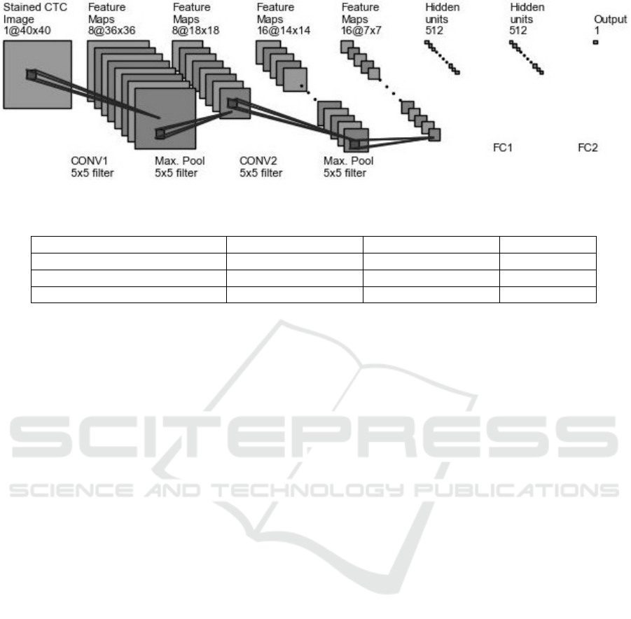
Figure 5: The ConvNet Architecture.

Table 3: Models Results.

Model Train Error Test Error Iterations

Multi Layer Perceptron 0.0364 6.1127 5,000

Convolutional Neural Network 0.0295 4.2822 5,000

Linear Regression 3.475 17.2613 5,000

the difference between predicted ( ˆy

(i)

) and actual va-

lues (y

(i)

∑

i=1



ˆy

(i)

− y

(i)



(3)

5 DISCUSSIONS

In this research, Convolutional Neural Network out-

performed both MLP and Linear regression with a

Root Mean Squared Error (RMSE) margin of 0.0069

and 3.4455 respectively on training error, and 1.8305

and 12.9791 respectively on test error. This perfor-

mance can be attributed to the fact that deep learning

models are capable of learning the best set of repre-

sentative features automatically. The learned feature

set is weighted and used to enumerate CTC’s given a

new sample instance.

Linear Regression model was trained on all the

pixel intensity values of the input image. It was

the worst performer just after MLP. The Multilayer

layer perceptron model outperformed Linear Regres-

sion with a variation of 3.4386 on train error and

11.146 on the test error. From this performance re-

cord it can be deduced that not all pixel intensity va-

lues are equally informative.

Manually generated features such as RGB histo-

gram or pixel intensity values though can represent

an instance, may require the expert to specify the right

set of features or extensive feature engineering techni-

ques thus expensive. Using all image pixel values is

an assumption that all pixel intensities are representa-

tive of an instance.

In contrary, the feature representations can be le-

arned automatically, on a low dimensional space du-

ring the training process. This is the core functional

and theoretical underpinning of deep learning models

such as Convolutional Neural Network. The deep le-

arning adoption was precipitated by the work done

by Krizhevsky et al. (2012). In the study, the re-

sult obtained halved error value for object recognition

during ImageNet competition. This was unpreceden-

ted performance record as Convolutional Neural Net-

work model outperformed all other classical simple

learning models used before. Following this, other

studies have extended the capability of classical Con-

vNet model leading to state-of-the art results in image

recognition (He et al., 2016), large scale image recog-

nition architectures Szegedy et al. (2015) and unpre-

cedented object detection performance Redmon et al.

(2016); Ren et al. (2015); Liu et al. (2016).

6 CONCLUSIONS

In this paper, we have presented a learning model

which can be used to enumerate Circulating Tumor

Cells (CTC’s) in a stained image sample. An algo-

rithm which extracts regions of interest was develo-

ped and based on the experiments carried out, Con-

volutional Neural Network outperformed both Linear

Regression and classical Multilayer Neural Network

architectures. This performance is attributed to the

fact that the preferred model had the potent to learn

intricate low level representative features on its own.

This is a unique characterization which have been at-

tributed to deep learning models such as ConvNet.

Circulating Tumor Enumeration using Deep Learning

301

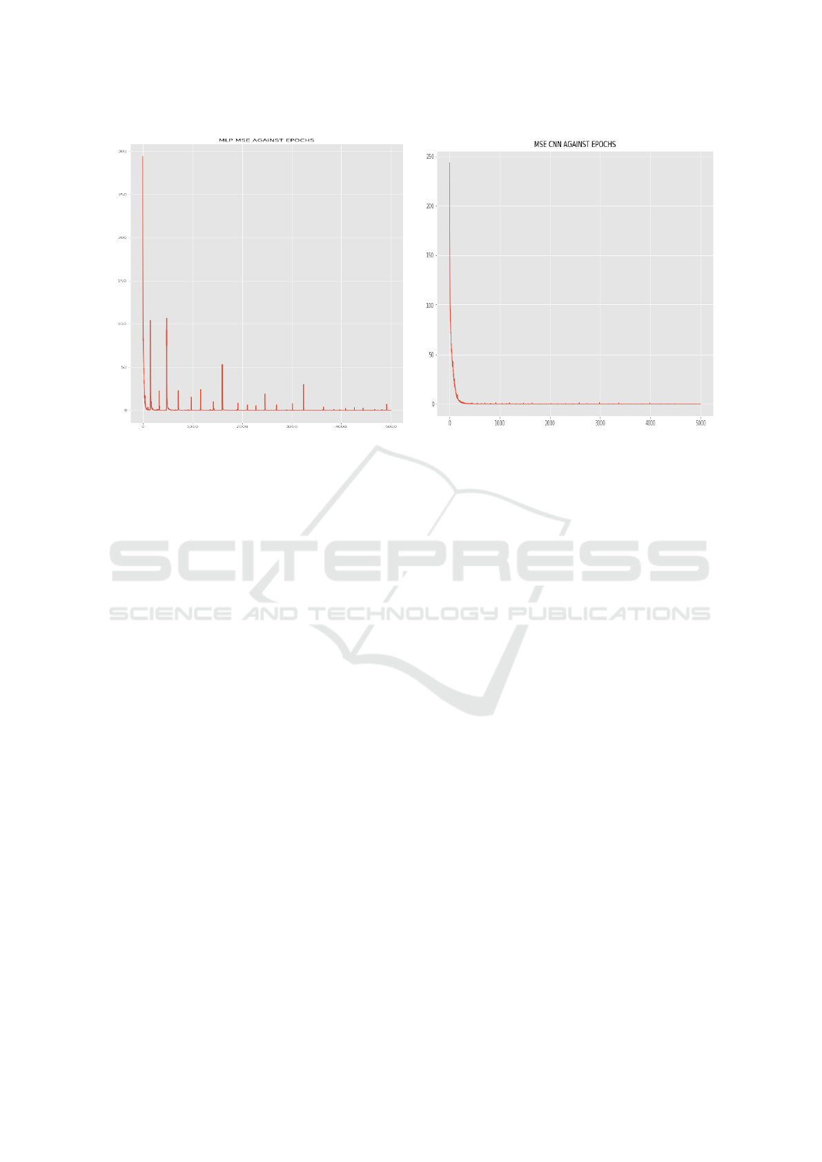
(a) MLPLoss (b) ConvNet Loss

Figure 6: MLP and ConvNet loss variations over epochs during training.

ACKNOWLEDGMENTS

The dataset used in this study was provided by Yunx-

iang Mao. He and others worked on a model which

only classiﬁes CTC’s instead of enumeration which is

presented in this paper.

REFERENCES

Crowley, E., Di Nicolantonio, F., Loupakis, F., and Bar-

delli, A. (2013). Liquid biopsy: monitoring cancer-

genetics in the blood. Nature reviews Clinical onco-

logy, 10(8):472–484.

Ferlay, J., H

ery, C., Autier, P., and Sankaranarayanan, R.

(2010). Global burden of breast cancer. In Breast

cancer epidemiology, pages 1–19. Springer.

Fitzmaurice, C., Dicker, D., Pain, A., Hamavid, H., Moradi-

Lakeh, M., MacIntyre, M. F., Allen, C., Hansen, G.,

Woodbrook, R., Wolfe, C., et al. (2015). The global

burden of cancer 2013. JAMA oncology, 1(4):505–

527.

Gonzalez, R. C. and Woods, R. E. (2002). Thresholding.

Digital Image Processing, pages 595–611.

He, K., Zhang, X., Ren, S., and Sun, J. (2016). Deep resi-

dual learning for image recognition. In Proceedings of

the IEEE conference on computer vision and pattern

recognition, pages 770–778.

Krizhevsky, A., Sutskever, I., and Hinton, G. E. (2012).

Imagenet classiﬁcation with deep convolutional neu-

ral networks. In Advances in neural information pro-

cessing systems, pages 1097–1105.

LeCun, Y., Bengio, Y., and Hinton, G. (2015). Deep lear-

ning. Nature, 521(7553):436–444.

Liu, W., Anguelov, D., Erhan, D., Szegedy, C., Reed, S., Fu,

C.-Y., and Berg, A. C. (2016). Ssd: Single shot mul-

tibox detector. In European conference on computer

vision, pages 21–37. Springer.

Mao, Y., Yin, Z., and Schober, J. (2016). A deep convoluti-

onal neural network trained on representative samples

for circulating tumor cell detection. In Applications of

Computer Vision (WACV), 2016 IEEE Winter Confe-

rence on, pages 1–6. IEEE.

Nielsen, M. A. (2015). Neural networks and deep learning.

Redmon, J., Divvala, S., Girshick, R., and Farhadi, A.

(2016). You only look once: Uniﬁed, real-time object

detection. In Proceedings of the IEEE conference on

computer vision and pattern recognition, pages 779–

788.

Ren, S., He, K., Girshick, R., and Sun, J. (2015). Faster

r-cnn: Towards real-time object detection with region

proposal networks. In Advances in neural information

processing systems, pages 91–99.

Scholtens, T. M., Schreuder, F., Ligthart, S. T., Swennen-

huis, J. F., Greve, J., and Terstappen, L. W. (2012).

Automated identiﬁcation of circulating tumor cells by

image cytometry. Cytometry Part A, 81(2):138–148.

Svensson, C.-M., Krusekopf, S., L

ucke, J., and Thilo Figge,

M. (2014). Automated detection of circulating tumor

cells with naive bayesian classiﬁers. Cytometry Part

A, 85(6):501–511.

Szegedy, C., Liu, W., Jia, Y., Sermanet, P., Reed, S., Angue-

lov, D., Erhan, D., Vanhoucke, V., and Rabinovich, A.

(2015). Going deeper with convolutions. In Procee-

dings of the IEEE conference on computer vision and

pattern recognition, pages 1–9.

IJCCI 2018 - 10th International Joint Conference on Computational Intelligence

302

Torre, L. A., Bray, F., Siegel, R. L., Ferlay, J., Lortet-

Tieulent, J., and Jemal, A. (2015). Global cancer

statistics, 2012. CA: a cancer journal for clinicians,

65(2):87–108.

Wang, D., Khosla, A., Gargeya, R., Irshad, H., and Beck,

A. H. (2016). Deep learning for identifying metastatic

breast cancer. arXiv preprint arXiv:1606.05718.

Circulating Tumor Enumeration using Deep Learning

303