
Research and Application of Array Dielectric Logging Tool
Zhiqiang Li
*
, Xinghai Gui, Zhiqiang Yang, Chen Li, Junyi Li and Yongli Ji
The 22nd Research Institute of China Electronics Technology Group Corporation.
Email:lizhiqiang316@126.com
Keywords: Array dielectric logging tool, lateral wave, finite-element, detecting depth, vertical resolution, thin interbed
layer
Abstract: Dielectric logging is an important tool in geophysical exploration. For formation with fresh water and where
water salinity is unknown, it has good performance in distinguishing oil and water layers. This paper
presents the calculation of electromagnetic field in layered medium by analytical formulas and by finite
element method, and compares the accuracy of these two methods. The inversion charts, measurements’
depth and vertical resolution are researched. The responses of thin layers and thin interbed layers are also
discussed. The designed array dielectric logging tool has been tested in practical wells. Research results
show that the analytical formulas are fast and effective for calculating apparatus response of layered
medium, and also for retrieving dielectric constant and resistivity. For the array dielectric logging tool, the
depth of investigation is 10-25cm, and the vertical resolution is 4cm. The array dielectric logging tool has
been tested in XX oil field. For freshwater formation with high resistivity, the measured dielectric constant
is about 10 in oil layers, and the measured dielectric constant is about 20 in water layers. The device could
distinguish oil and water layers obviously, which offer additional method for formation evaluation.
1 INTRODUCTION
Daev proposed high frequency logging method. The
method aimed to measure the phase difference of
two receiving coil, under the radiation of
electromagnetic wave by transmitting coil. When the
working frequency is about several tens of gigahertz,
phase difference is mainly due to dielectric constant
of rocks. Several Institutes, such as Moscow
Institute of Geology, Siberian Branch of the Russian
Academy of Sciences and Geophysical Institute,
performed a lot of work on high frequency logging.
They finished the theoretical research, developed the
experimental prototype, and did experiment in wells.
The high frequency logging began its commercial
production. By then, a new method arose in the field
of electric logging, which is measuring the dielectric
constant and conductivity of rocks by
electromagnetic waves at from several hundreds of
kilohertz to several of gigahertz (Hizem et al., 2008;
Freedman and Grove, 1990; Seleznev et al., 2006).
Dunn deduced the formula of lateral wave
excited by horizontal electric dipole in three
horizontal layers (Dunn, 1986). Wu Xinbao obtained
the iterative method of calculating the lateral wave
excited by horizontal magnetic dipole in two
horizontal layers (Wu and Pan, 1992; Wu and Pan,
1990). Chew proposed numerical model-matching
method(NMM) in calculating the response of
vertical magnetic dipole in cylindrical layers (Chew
and Gianzero, 1981). Liu Manfen deduced the
formula of the response of arbitrary oriented dipole
in dielectric media (Liu et al., 1994).
2 FORMULAS OF LATERAL
WAVES IN LAYERED MEDIA
2.1 Electromagnetic Fields in
Spherical Coordinates within
Homogenous Media
The electromagnetic fields within homogenous
media are
=−
(
1+
)
4
(1)
=−
(
1+
)
2
(2)
in which, is angular frequency, is magnetic
permeability, r is the radius of receiving coil, L is
the distance between transmitting point to receiving
point, M is the magnetic dipole moment of
transmitting coil. =
−(+)
is wave
406
Li, Z., Gui, X., Yang, Z., Li, C., Li, J. and Ji, Y.
Research and Application of Array Dielectric Logging Tool.
In Proceedings of the International Workshop on Environment and Geoscience (IWEG 2018), pages 406-414
ISBN: 978-989-758-342-1
Copyright © 2018 by SCITEPRESS – Science and Technology Publications, Lda. All rights reserved
number, where is electrical conductivity of
formation, is dielectric constant of formation.
2.2 Formulas of Lateral Waves in
Horizontally Layered Media
According to the former research results, the size,
curvity and electrical conductivity of probe plate
could be omitted. So the transmitting antenna could
be equivalent to magnetic dipole. The problem is
reduced to electromagnetic field excited by magnetic
dipole in horizontally layered media.
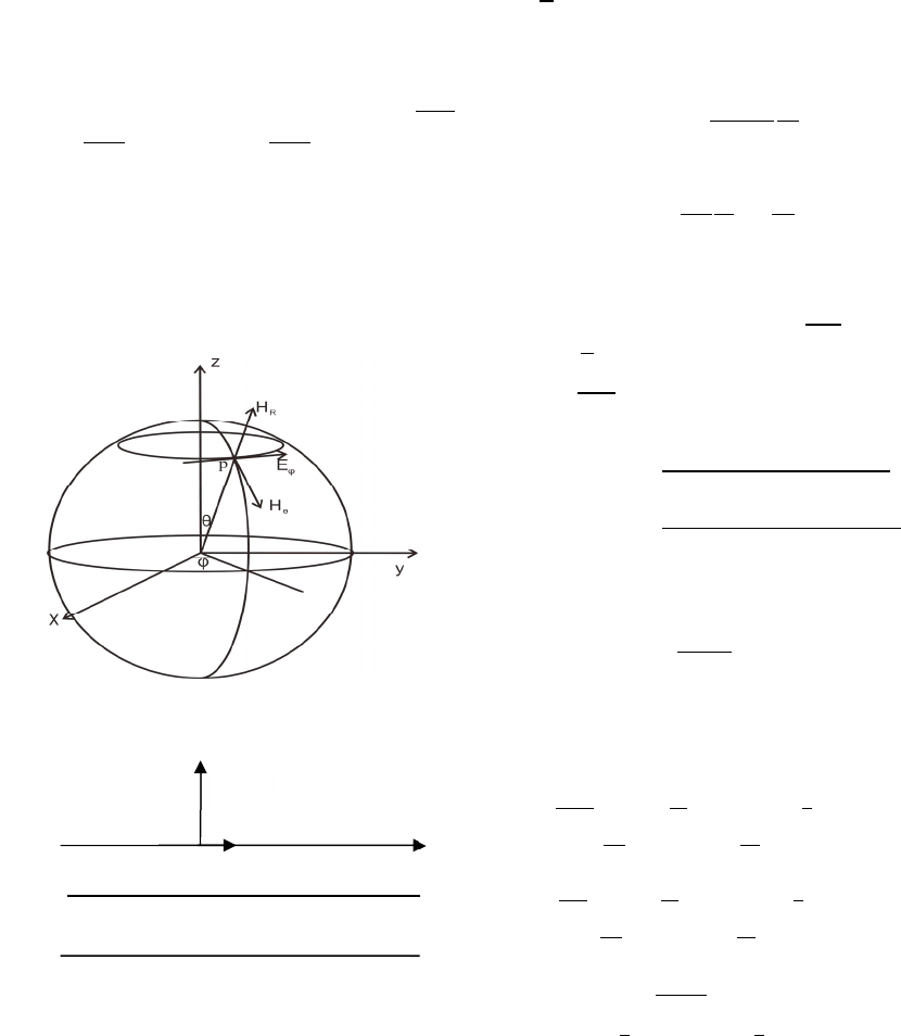
As in Figure 2, region 1 is mud cake, region 2 is
flushed zone, region 3 is undisturbed zone, in which
the wave numbers respectively are
=
̃
,
=
̃
, and
=
̃
, in which is
angular frequency,
,
and
are the magnetic
permeability in region 1, region 2 and region 3, and
̃
, ̃
and ̃
are the complex dielectric constants in
region 1, region 2 and region 3. The horizontal
magnetic dipole is at the origin point, in the
direction of x, and with magnetic dipole moment of
M, See Figure 1.
Figure 1: Magnetic dipole in spherical coordinates.
Figure 2: Model of dielectric logging.
From Maxwell’s equations, we know:
∇×
=
+
∇×
=−
̅
∇∙
=0
∇∙
=−
∇∙
(3)
in which
=
(
)
(
)
(
+
)
=1
0=2,3
, where m is the equivalent magnetic dipole moment
of the antenna. In cylindrical coordinate,
=
(
)
(
)
(
+
)
=1
0=2,3
. From Equation
3, we get the expression of z component of
electromagnetic field in cylindrical coordinate:
(
∇
+
)
=−
−
(
)
(
+
)
(
∇
+
)
=0
(
∇
+
)
=0
(4−A)
(
∇
+k
)
B
=
μ
m
ρ
d
dρ
δ
(
ρ
)
d
dφ
δ
(
φ
)
δ
(
z+z
)
(
∇
+k
)
B
=0
(
∇
+k
)
B
=0
(4−B)
Using Fourier transformation,
and
are
obtained as:
=
sin
cos
−
cos
(
)
(
5
)
=
2
cos
sin
−sin
(
)
(6)
in which,
=
(+)
cos
(
)
+sin
(
)
=
(
+
)
sin
(
)
+sin
(
)
=
̅
(
̅
−
̅
)
(
)
+
(
̅
+
̅
)
(
)
=
̅
(
̅
−
̅
)
(
)
−
(
̅
+
̅
)
(
)
=
(
−
)
(
)
+
(
+
)
(
)
=
(
−
)
(
)
−
(
+
)
(
)
=
−
(
=1,2,3
)
Expand Maxwell’s equation shown in Equation 3
into individual components in cylindrical form, and
according to Equation 5 and Equation 6, the other
components of electromagnetic fields are:
=
−
2
cos −
2
(
)
+
(
)
−
2
(
)
−
(
)
cos
+
2
(
)
+
(
)
+
2
(
)
−
(
)
cos
(7)
=
2
sin −
2
(
)
−
(
)
−
2
(
)
+
(
)
cos
+
2
(
)
−
(
)
+
2
(
)
+
(
)
cos
(8)
=
−
2
sin
(
)
sin
(
)
−
2
(
)
−
(
)
+
2
(
)
+
(
)
sin
(9)
conductive
l
zone 1
zone 2
x
z
M
zone 3
Research and Application of Array Dielectric Logging Tool
407

=
2
cos
(
)
sin
(
)
−
2
(
)
+
(
)
+
2
(
)
−
(
)
sin
(10)
When =0,
=
−
2
cos −
2
(
)
+
(
)
−
2
(
)
−
(
)
+
2
(
)
+
(
)
+
2
(
)
−
(
)
(11)
=
2
sin −
2
(
)
−
(
)
−
2
(
)
+
(
)
+
2
(
)
−
(
)
+
2
(
)
+
(
)
(12)
=
sin
1−
(
)
(13)
in which the component of electromagnetic
fields is received by antenna vertical to well axis,
and at the same time =0°. The component of
electromagnetic fields is received by antenna
parallel to well axis, and at the same time =90°.
For the two array antennas, we introduce the
amplitude attenuation A(dB) and phase shift ∆
=8.686×
(13)
∆=
×
(14)
2.3 Finite Element Method in Dielectric
Media
According to electromagnetic theory and
computational electromagnetic, the problem of
electric field may come down to the following
functional extremum problem (Zhang, 1986;
Dhayalan et al., 2018; Chen et al., 2017):
=
∭
∙
−∇×
+
∙
(15)
∇×
=
(16)
After the discretization of the 3-dimentional
formation, stiffness matrix is obtained. Using
iterative algorithm, the 3-dimentional response of
array dielectric logging tool could be calculated. The
detailed content about this could be found in various
monographs, so no need to be repeated here.
3 ANALYSIS ON THE
CALCULATED RESULTS
3.1 Compare the Calculated Results
Case 1: homogeneous space with dielectric constant
of 1, the magnetic permeability of 1, and electrical
conductivity from 1e-3S/m to 1S/m. The distance
between transmitting and receiving antenna is
0.14m.
Magnetic dipole and Lateral wave are two
different analytic methods.
Case 2: homogeneous space with dielectric
constant from 10 to 80, the magnetic permeability of
1, and electrical conductivity from 0.1S/m. The
distance between transmitting and receiving antenna
is 0.14m.
From Table 1 and Table 2, we can see that the
results of lateral wave and magnetic dipole is
consistent. And under the influence of meshing, the
finite element method has an error about 5%.
Table 1: Results in homogeneous formation with different conductivity.
Method
σ s/m
1e-3 1e-2 1e-1 1
Hz (Magnetic dipole) 45.5-348.2i 59.4-279.6i 61.3-23.92i 0.123-0.26i
Hz (Lateral wave) 45.1- 348.3i 59.3-279.7i 61.3-23.97i 0.123-0.26i
Hz (Finite element) 46.9-348.7i 59.6-280.0i 61.2-23.6i 0.128-0.26i
Hx (Magnetic dipole) -455.0+82.6i -360.4+132.8i 28.03+133.6i -0.669+1.70i
Hx (Lateral wave) -455.03+ 82.5i -360.3+132.7i 28.02+133.6i -0.669 + 1.70i
Hx (Finite element) -454.9+82.4i -360.8+133.0i 28.38+133.8i -0.628+1.72i
IWEG 2018 - International Workshop on Environment and Geoscience
408
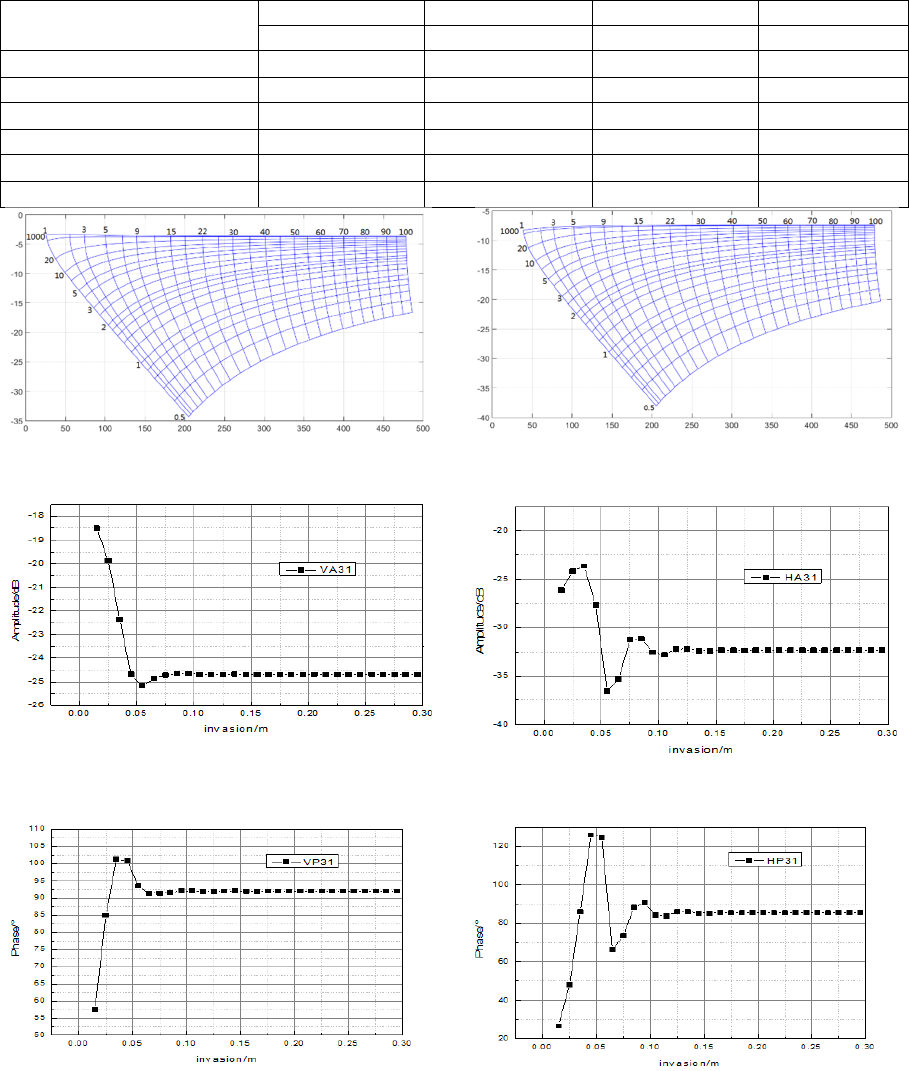
Table 2: Results in homogeneous formation with different dieletric constant.
Method
10 30 50 80
Hz (Magnetic dipole) 40.1-478.0i 518.4-1034.6i 1530.4-646.0i 2084.6+894.3i
Hz (Lateral wave) 40.2 - 478.1i 514.1-1036.9i 1533.8- 638.2i 2079.9+908.2i
Hz (Finite element) 39.8- 478.8i 512.2-1037.6i 1535.3- 634.6i 2076.9+914.2i
Hx (Magnetic dipole) -2184.5+390.1i -8170.4+4386.1i -6936.4-1574.2i 11505-27436i
Hx (Lateral wave) -2185.0+388.8i -8177.4+4369.3i -6894.3-15755i 11591-27387i
Hx (Finite element) -2185.1+386.5i -8182.8+4353.6i -6856.9-15767i 11669-27345i
Figure 3a: Inversion chart of vertical polarization. Figure 3b: Inversion chart of horizontal polarization.
Figure 4a: Amplitude ratio of vertical polarization. Figure 4b: Amplitude ratio of horizontal polarization.
Figure 4c: Phase shift of vertical polarization. Figure 4d: Phase shift of horizontal polarization.
Figure 4: Detecting depth when resistivity of flushed zone is low.
Research and Application of Array Dielectric Logging Tool
409
3.2 Inversion Chart
By calculation, the inversion chart of the two
different polarization antenna is obtained as in
Figure 3.a and Figure 3.b, in which the lateral axis is
phase difference, and the longitude axis is amplitude
ratio. The dielectric constant is from 1 to 100, and
the electrical resistivity is form 0.5 to 100Ω·m.
3.3 Detecting Depth
Case 1: Mud cake is with thickness of 0.5cm,
dielectric constant of 25, conductivity of 1S/m, and
flushed zone is with dielectric constant of 20,
conductivity of 0.6S/m, and undisturbed zone is with
dielectric constant of 15, conductivity of 0.3S/m.
Detecting depth is evaluated by the phase difference
and amplitude ratio between the nearest and farthest
receiving antennas.
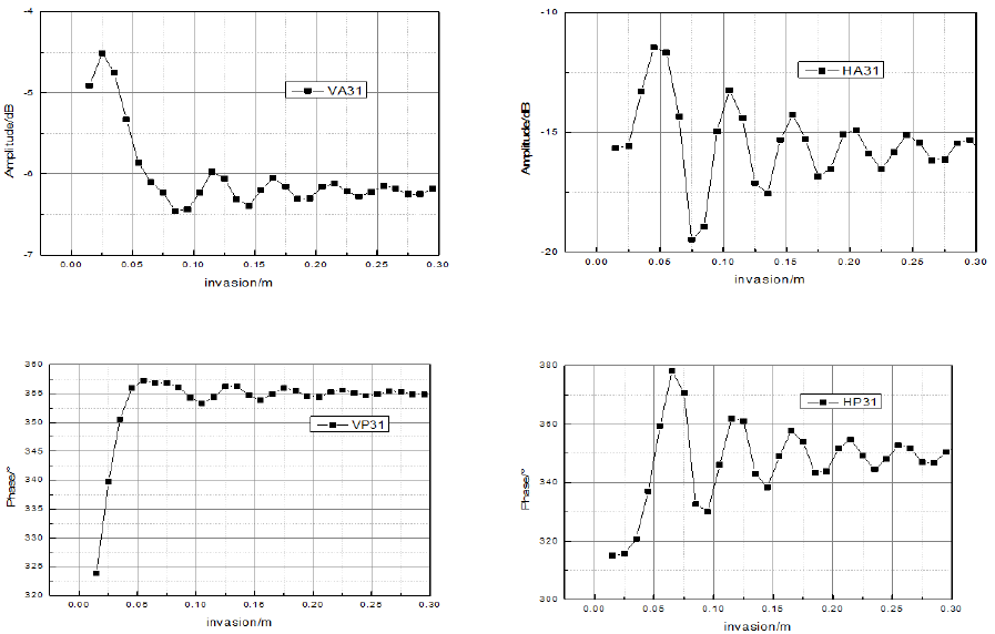
Case 2: Mud cake is with thickness of 0.5cm,
dielectric constant of 60, conductivity of 0.25 S/m,
and flushed zone is with dielectric constant of 12,
conductivity of 0.033S/m, and undisturbed zone is
with dielectric constant of 9, conductivity of
0.01S/m.
From Figure 4 and Figure 5 it is seen that, in
formation with flushed zone of low resistivity, when
the radius of flushed zone is larger than 6cm, phase
shift and amplitude ratio of vertical polarization do
not have obvious changes, which indicate that
deeper formation can’t be detected. For horizontal
polarization, when the radius of flushed zone is
larger than 6cm, deeper formation can’t be detected.
In formation with flushed zone of low resistivity,
when the radius of flushed zone is larger than 20cm,
phase shift and amplitude ratio of vertical
polarization do not have obvious changes, and when
the radius of flushed zone is larger than 30cm, phase
shift and amplitude ratio of horizontal polarization
do not have obvious changes. According to these
simulated results, it is seen that detecting depth of
horizontal polarization is larger than detecting depth
of vertical polarization.
Figure 5a: Amplitude ratio of vertical polarization. Figure 5b: Amplitude ratio of horizontal polarization.
Figure 5c: Phase shift of vertical polarization. Figure 5d: Phase shift of horizontal polarization.
Figure 5: Detecting depth when resistivity of flushed zone is high.
IWEG 2018 - International Workshop on Environment and Geoscience
410
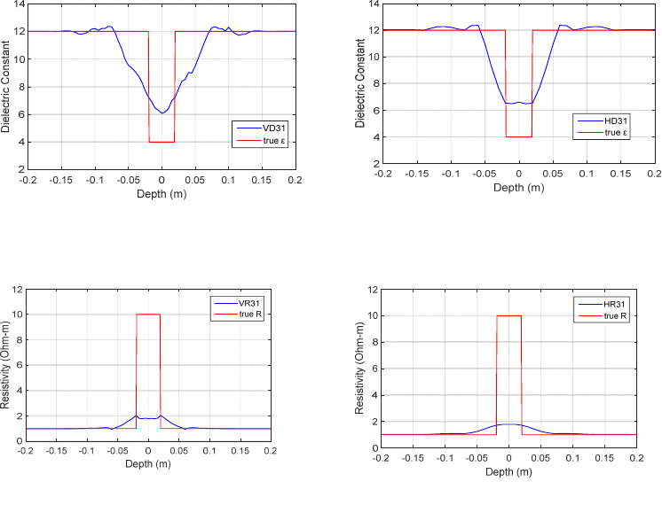
Figure 6a: Dielectric response of vertical
polarization.
Figure 6b: Dielectric response of horizontal
polarization.
Figure 6c: Resistivity response of vertical
polarization.
Figure 6d: Resistivity response of horizontal
polarization.
3.4 Vertical Resolution
From these response curves as shown in Figure 6, it
is seen that in layer with thickness of 4 cm, the
apparent dielectric constant is about 6. The array
dielectric logging tool is able to distinguish thin
layers with thickness of 4 cm, showing the relative
high vertical resolution.
4 APPLICATION IN THE
PRACTICAL WELLS
Guguba well located at the south rim of Island, with
well depth of 2800.80m, and the technical casing is
244.5mm, setting at depth 1945.65m (the Ordovician
submarine mountain interface), under which is
borehole drilling by 216.0mm drilling bit. Formation
of Ordovician and Cambrian is mainly limestone and
dolostone. The apertures are well-developed. There
are reservoirs of class I, II and III. Porosity
distribution is 3-20%. Resistivity of shale is 5-6Ω·m.
Resistivity of dense layer is 1000-2000Ω·m.
Resistivity of developed apertures is 8-60Ω·m.
Abundant logging data is beneficial to evaluate new
logging results.
1). From Figure 7 it is seen that, the dielectric
curve and resistivity curve show good antisymmetry
in dielectric logging data, and agree with the true
formation.
2). The dielectric curve and resistivity curve
show good response to thin layers and thin interbed
layers in dielectric logging data, and are in good
agreement with data from micro-scanner logging.
3). From Figure 8 it is seen that,at the depth of
700 m – 710m of XX well, water layer show low
resistivity and high dielectric constant.
4). From Figure 8 it is seen that,at the depth of
762.6 m – 774m of XX well, three reservoir layer
show slightly high resistivity in conventional
logging curves, and are more evaluated as water
layers. But in dielectric logging results, the dielectric
curves are different in the three reservoir layer, layer
5 and layer 6 should more accurately be evaluated as
oil-water layers.
5). Layer 10 and layer 11 in XX well, with
resistivity of 10Ω·m, are evaluated as oil according
to data of adjacent wells. From dielectric logging
results, the dielectric constants are quite low, about
10, which clearly indicate oil layers.
Research and Application of Array Dielectric Logging Tool
411

Figure 7a: Comparison between dielectric and resistivity logging data.
Figure 7b: Comparison between dielectric and micro-scanner logging data in thin layers.
Figure 7c: Comparison between dielectric and micro-scanner data in thin interbed layers.
Frozen picture
Depth
Frozen picture
Depth
IWEG 2018 - International Workshop on Environment and Geoscience
412
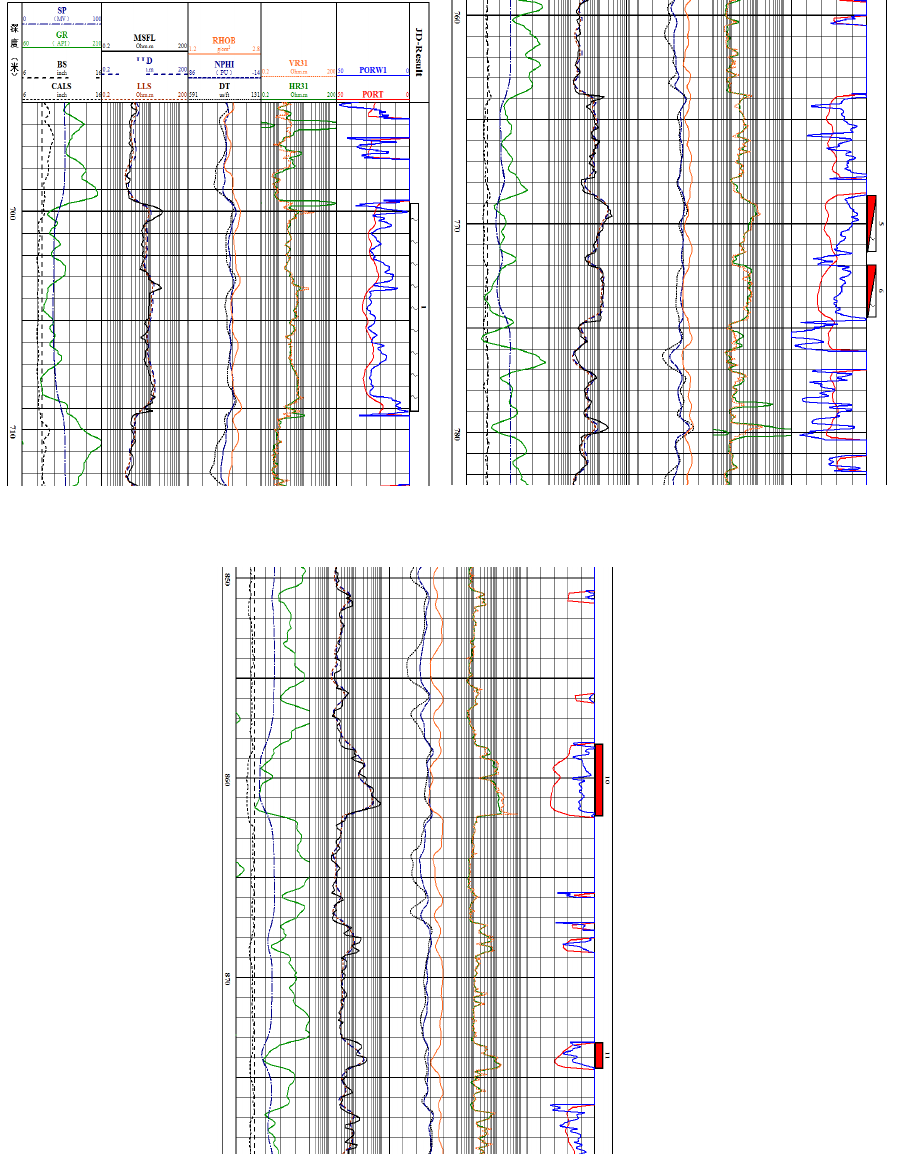
Figure 8a: Dielectric response to water layer in XX well. Figure 8b: Dielectric response to oil-water layer in XX well.
Figure 8c: Dielectric response to oil layer in XX well.
Research and Application of Array Dielectric Logging Tool
413
5 CONCLUSIONS
1) Analytical solution is obtained in horizontally
layered media, and is compared with homogenous
formation. Through three dimensional simulation by
finite element method, it is seen that the two
methods are reliable and with high accuracy.
2) According to the detecting performance of the
dielectric logging tool, vertical resolution is 0.04 m,
illustrating that thin layers and thin interbed layers
can be effectively distinguished. The detecting depth
can reach up to 0.1-0.25 m.
3) Array dielectric logging tool is able to detect
resistivity and dielectric constant in both vertical
and horizontal direction.
4) In formation with fresh water, resistivity are
both high in water layer and oil layer. Using
dielectric logging one can make effective
evaluation.
REFERENCES
Chen R, Kuang X, Li Z 2017 Numerical computation of
infinite Bessel transforms with high frequence
International Journal of Computer Mathematics
Chew W C and Gianzero S C 1981 Theoretical
investigation of the electromagnetic wave propagation
tool IEEE Trans. Geosci. Remote Sens 19(1)
Dhayalan R, Kumar A, Rao BP 2018 Numerical analysis
of frequency optimization and effect of liquid sodium
for ultrasonic high frequency guided wave inspection
of core support structure of fast breeder reactor Annals
of Nuclear Energy
Dunn J M 1986 Lateral wave propagation in a three-
layered medium Radio Science 21
Freedman R and Grove G P 1990 Interpretation of EPT-G
logs in the presence of Mudcake SPE Formation
Evaluation 5(04)
Hizem M, Budan H, Deville B, and et al 2008 Dielectric
dispersion: A new wire line petrophysical
measurement SPE Annual Technical Conference and
Exhibition
Liu M F, Feng G Q, Wang X J, et a l 1994 Theoretical
Investigation of Shoulder Bed Thin Sandwich Effect
and Vertical Resolution for The High Frequency
Dielectric Logging Chinese Journal of Geophysics 37
Seleznev N V, Habashy T M, Boyd A J, et al 2006
Formation properties derived from a multi-frequency
dielectric measurement SPWLA 47th Annual Logging
Symposium
Wu X B and Pan W Y 1990 New Formulas for the Lateral
Waves of HMD in a Three-Layered Medium Chinese
Journal of Radio Science 5(3)
Wu X B and Pan W Y 1992 The Lateral Wave
Propagation in Electromagnetic Wave Propagation
Log Chinese Journal of Geophysics 35(1)
Zhang G J 1986 Electrical Logging, PetroIeum Industry
Press,
IWEG 2018 - International Workshop on Environment and Geoscience
414
