
The Method of Engine Fault Diagnosis Based on Improved SVM
Tongfei Shang
1
, Wei Chen
2
and Kun Han
3
1
College of Electronics and Information Engineering, Xi'an Jiaotong University, Xi'an, China
2
Department of Aviation Ammunition Support, Air Force Logistics Support, Xuzhou, China
3
College of Information and Communication, National University of Defense Technology, Changsha, China
Keywords: SVM; Engine; Fault diagnosis.
Abstract: The paper aimed at the common reasons of engine fault, established the membership matrix between the
symptoms of the engine fault and the fault modes, and used optimized fault diagnosis model established to
perform intelligent fault diagnosis, the simulation analysis proved the effectiveness of proposed method.
1 INTRODUCTION
Because of the excellent performance and strict
theoretical basis of SVM, many improved SVM
algorithms have been proposed[1-3]. The paper used
GA algorithm to optimize the parameters of SVM,
then made the fault diagnosis model based on
classified SVM, to diagnose the engine fault, finally
examples were used to verify the effectiveness of
model.
2 FAULT DIAGNOSIS MODEL
BASED ON REGRESSION
SUPPORT VECTOR MACHINE
For regression-type support vector machines, we
first consider using a linear regression function
bxwxf +⋅=)(
to fit the data },{
ii
yx ,
ni ,,1 K=
,
d
i
d
i
RyRx ∈∈ ,
, so that the
function regression problem can be described as how
to find a function
f
∈
F that minimizes the loss
function. The commonly used loss functions[4]
are:
quadratic loss function, Huber loss function, and
ε
-
insensitivity loss function, where the
ε
-insensitivity
loss function is an approximate form of the Huber
loss function proposed by Vapnik due to its unique
sparseness. In general, the solution to the
ε
-
insensitivity loss function has the least number of
support vectors used in the expansion of the solution
and is therefore widely used.
ε
-Insensitive loss function is defined as:
⎪
⎩
⎪
⎨
⎧
−−
≤−
=
Otherwxfy
wxfy
l
ε
ε
),(
),(0
(1)
Among them,
w
for the parameters to be
identified,
ε
given accuracy.
The regression estimation problem is defined as
the problem of minimizing the risk of a loss
function. When using the SRM principle to
minimize the risk, the optimal regression function is
to minimize the functional under certain constraints,
when using - insensitive loss For functions, the
minimization constraint is
ni
ybxw
bxwy
ii
ii
,,1 L=
⎩
⎨
⎧
≤−+⋅
≤−⋅−
ε
ε
(2)
The optimization goal is minimization
2
2
1
w
,
and statistical learning theory points out that under
this optimization goal, better promotion ability can
be achieved. Considering the case where the fitting
error is allowed, if the relaxation factor
i
ξ
≥0 and
∗
i
ξ
≥0, are introduced, the above equation becomes

ni
ybxw
bxwy
ii
ii
,,1 L=
⎩
⎨
⎧
+≤−+⋅
+≤−⋅−
ξε
ξε
(3)
The optimization goal is minimized:
∑
=
∗
++
n
i
ii
Cw
1
2
2
1
ξξ
, where the constant C > 0, C
denotes the degree of penalty for samples that
exceed the error
ε
. This is a convex quadratic
optimization problem, introducing the Lagrange
function:
∑∑
∑∑
=
∗∗
=
∗
==
∗∗
+−−⋅−++−
−⋅−++−++=
r
i
iiiiiii
r
i
i
iii
r
i
i
r
i
iii
bxwya
bxwyaCwwL
11
11
1
2
)()(
)()(
2
1
),,(
ξηξηξε
ξεξξξξ
(4)
Where,
i
a and
∗
i
a
are Lagrange factors. Using
the optimization method can get its dual problem
))(()(
2
1
)()(),(:
111
jijj
n
i
ii
n
i
iii
n
i
ii
xxaaaaaayaaaaWMax ⋅−−−−++−=
∗
=
∗
=
∗
=
∗∗
∑∑∑
ε
(5)
niCaaaats
ii
n
i
ii
,,1,,0,0)(..
1
L=≤≤=−
∗
=
∗
∑
The aggression function is:
∗
=
∗
+⋅−=+⋅=
∑
bxxaabxwxf
i
n
i
ii
)()()(
1
(6)
Among them,
i
a and
∗
i
a
, only a small part is not 0,
their corresponding sample is the support vector.
3 SUPPORT VECTOR MACHINE
PARAMETER OPTIMIZATION
In order to improve the classification performance of
SVM, training and testing samples are needed to
determine the kernel parameters and penalty factors
of the optimal SVM. The use of genetic algorithm
can quickly search out the globally optimal
parameter value, which not only saves the search
time, but also improves the classification
performance. In the process of classification using
support vector machines, the main parameters
affecting the classification performance of the
support vector machine include: penalty function C
and kernel function parameters[5].
3.1 Genetic Coding And Fitness
Function Design
3.1.1 Coding Method And Coding Range
The loss function parameter ε, the penalty factor C,
the kernel width
σ
of the radial basis kernel
function, and the embedding dimension
p
of the
time series are all coded using floating-point number
coding. The coding interval is the value interval of
each parameter.
3.1.2 Design of fitness function
In order to evaluate the prediction effect and
accuracy of the model, the root mean square relative
error (RMSRE) can be used to measure the accuracy
of the prediction. The smaller the root mean square
relative error, the higher the accuracy of the
prediction.
∑
=
⎟
⎟
⎠
⎞
⎜
⎜
⎝
⎛
−
−
=
N
nt
t
ltt
tr
l
tr
y
yy
nN
RMSRE
2
,
ˆ
1
(7)
In the formula,
tr
n
is the number of training
samples, N is the sample size, and
lt
y
,
ˆ
is the
prediction result of the department
l
. The fitness
function is expressed as
l
RMSRE
Fit
1
)PC( =、、、
σε
(8)
3.2 Genetic Operation
3.2.1 Select Operation
Use fitness sorting method. First, the individuals in
the population are sorted according to the fitness
value. Then determine the probability of the ⅰth
individual being selected by
]
1
1
)([
1
−
−
−−=
M
i
baa
M
P
i
(9)
In the formula, M is the number of individuals in
the population, P
i
is the individual's probability of
selection, satisfies
∑
=
M
i
i
P
1
= 1, and P1≥P2≥P3≥P4
≥...≥PM, i is the serial number of the individual, 1
≤a≤2 , b=2-a.
3.2.2 Cross Selection
The crossover operation uses a linear combination.
When you cross-operate a certain probability on a
certain two chromosomes X1 and X2, you can use
the following method:
X
1
=uX
1
+(1-u)X
2
; (10)
X
2
=(1-u)X
1
+uX
2
; (11)
In the formula, μ=U(0,1) is a random number
between 0 and 1.
3.2.3 Mutation Operation
The mutation operator used is as follows: randomly
select a mutation bit j in the chromosome to be
mutated, and set it as a normalized random number
U(a
i
, b
i
). a
i
, b
i
is the upper and lower limits of the
corresponding mutation:
⎩
⎨
⎧
=
=
otherwisex
jiifbaU
X
i
ii
j
),(
(12)
4 SIMULATION
There are six common automatic engine fault
symptoms for an engine, namely, exhaust
temperature over-temperature (F1), vibration (F2),
speed drop (F3), oil warning light (F4), and large oil
consumption ( F5) and speed does not go up (F6),
there are 5 causes of failure, namely centrifugal
valve axis (S1), turbine blade fracture (S2), oil
pipeline rupture (S3), oil pump follow-up piston
stuck (S4 And the drive shaft is broken (S5). After
establishing the membership matrix between the
fault symptoms and the failure modes, the intelligent
fault diagnosis is performed using the optimized
fault diagnosis model established in this paper.
After obfuscation and determination by
experienced experts, the membership relationship
between the symptoms of the failure and the cause
of the fault is shown in Table 1. After the feature
information is obtained, the support vector can be
trained. At the same time, in order to verify its
robustness and anti-jamming performance, different
Gaussian noises were added. The classification
results obtained are shown in Tables 2 and 3. (Table
2 shows the network diagnostics when the noise
reaches 0.15, where 1,2,3 , 4, 5 for the indication of
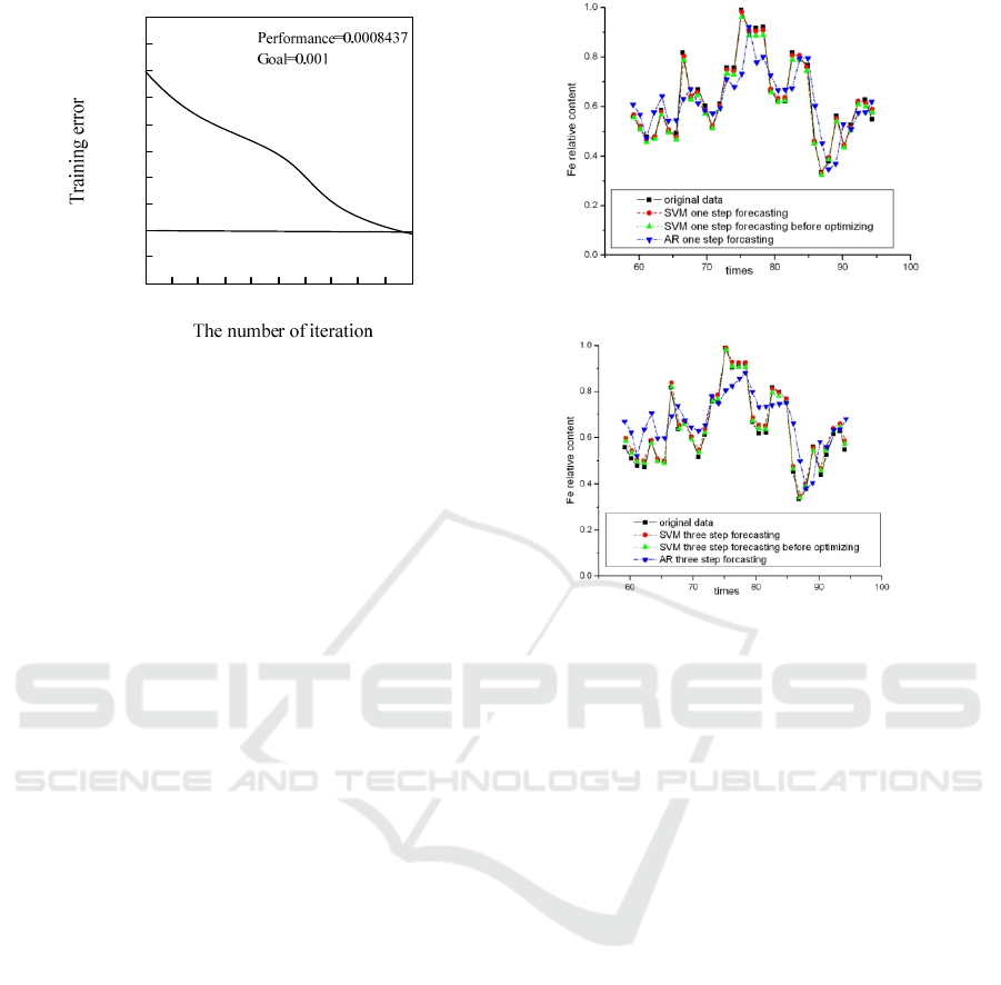
the corresponding failure mode). Figure 1 shows the
error curve for network training. From Table 2,
Figure 1 can be seen: 1 in the case of noise, the
classification accuracy of the classification support
vector machine is higher; 2 convergence speed is
very fast (11 steps to reach the error requirements).
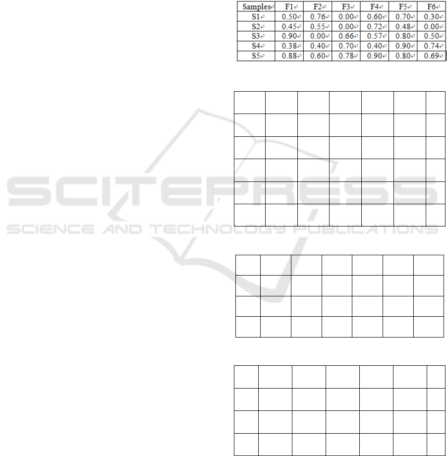
Table 1: Engine fault training samples.
Table 2: The training result under the 0.15Gaussian noise.
Fault
mode
Fault
type
Fault1 0.8806 -0.5780 -0.4575 0.5147 -0.3570 4
Fault2 0.1264 0.3006 0.0142 0.6696 -0.5254 1
Fault3 0.2575 -0.1228 1.1453 0.1481 -0.0430 2
Fault4 0.2201 -0.4717 0.3056 1.2915 -0.4647 3
Fault5 0.8251 -0.5221 0.4017 0.4511 0.3236 4
Table 3: Testing fault samples.
Fault
mode
F1 F2 F3 F4 F5 F6
T1 0.66 0.73 0.98 0.08 0.23 0.40
T2 0.20 0.57 0.60 0.77 0.25 0.66
T3 0.43 0.25 0.61 0.34 0.15 0.46
Table 4: Classified results.
Fault
mode
Fault
type
T1 0.2001 -0.1105 1.0145 0.1585 -0.1002 2
T2 0.8220 -0.5441 0.3996 0.4258 0.3002 4
T3 0.1002 0.3548 0.0787 0.6102 -0.5003 1
24
6
8
10
3
10
−
4
10
−
2
10
−
1
10
0
10
1
10
−
Figure 1: Training error curve.
In this type of engine, several times of automatic
parking parameters were collected during several
test runs. After filtering and processing, six
symptom parameters are extracted. These
parameters are subjected to fuzzy processing by the
selected membership function (preprocessing of the
input signal of the type-class support vector
machine) to obtain the fuzzy feature vector as shown
in Table 3 and substituted into the training. The test
is performed in a good support vector network. The
diagnosis results are shown in Table 4. These three
faults were manually diagnosed by field experts and
were diagnosed as: T1 centrifugal valve holding
shaft (S1), T2 lubricating pipe vibration (S3) and T3
drive shaft broken (S5). It can be seen from the
above that the accuracy of the fault diagnosis model
based on the subdivision type support vector
machine based on fault diagnosis is 100%, which
shows that the model is really efficient and practical
for fault diagnosis.
Finally, using training and test results, the data is
divided into two groups: the first 60 data as training
data, and the last 34 as test data. In the calculation
process, in order to analyze the accuracy of the
forecasting model of the optimized SVM state
forecasting model, AR model, SVM model, and
optimized SVM model are used to predict one step
and three steps in advance. As shown in Figures 2
and 3, the prediction accuracy of the support vector
machine optimized by the genetic algorithm is better
than that of the support vector machine based on
empirical selection of each parameter.
Figure 2: The prediction result of one step in advance.
Figure 3: The prediction result of three step in advance.
5 CONCLUSIONS
The paper introduced the basic theory of SVM,
constructed the fault diagnosis model based on
classified SVM, used the GA algorithm to optimize
and select the parameters of SVM, the simulation
proved the proposed algorithm to be effective,
robust and correct, provided a powerful guarantee
for effective and real-time monitoring of the engine.
REFERENCES
1. Francis E H Tay,Lijuan Cao.Application of support
vector machines in financial timeSeries
forecasting[J].Omega,2011(29):309~317
2.
Vladimir Cherkassky,Ma Yunqian.Practical selection
of SVM parameters and noise estimation for SVM
regression[J].NeuraNetworks,2014(17):113~126
3.
Theodore B T,Huseyin I.Support vector machine for
regression and application to financial forecasting[J]
.
Proceeding of the IEEE-INNS-ENNS International
Joint Conference on Neural Network,2000(6):348~353
4.
Steve R. Support vector machines for classification
and regression [D]. 2004,University of Southampton
5.
Baker J.E.. Adaptive selection methods for genetic
algorithms[J], Proc. of the Intel Conf. on Genetic
Algorithms and Their Applications, 2008:101~111
