Research and Application of Target Tracking Algorithm
Bailin Lin
1
, Zheng’an Xiao
1
School of Physics and Mechanical
﹠
Electrical Engineering, Hubei University of Education, Wuhan, China
Keywords: Particle filter, mean shift, target tracking.
Abstract: This paper studies the principle of particle filtering and mean shift algorithm, analyzes the influence of
particle number on particle filter, and carries out tracking experiments on the target of the sports ship. Using
the method of polynomial fitting, the actual motion trajectory of the ship was manually sampled and
compared with the method trajectory of this article. The real-time performance of the algorithm is analyzed
and the experimental results are given.
1 INTRODUCTION
The purpose of video target tracking is to analyze
the video sequence captured by the sensor and
correlate the same moving target in different frames
of the image sequence to obtain the complete motion
track of each moving target. The essence of target
tracking is to analyze the video sequence captured
by the image sensor and calculate the position, size
and movement speed of the target in each frame of
the image. As a main branch of the field of computer
vision, the research of video target tracking method
is increasingly applied to security, intelligent video
surveillance, intelligent traffic management, military
robot vision and other fields. This article takes sports
ship target tracking as an example to carry out
relevant algorithms and experimental research. The
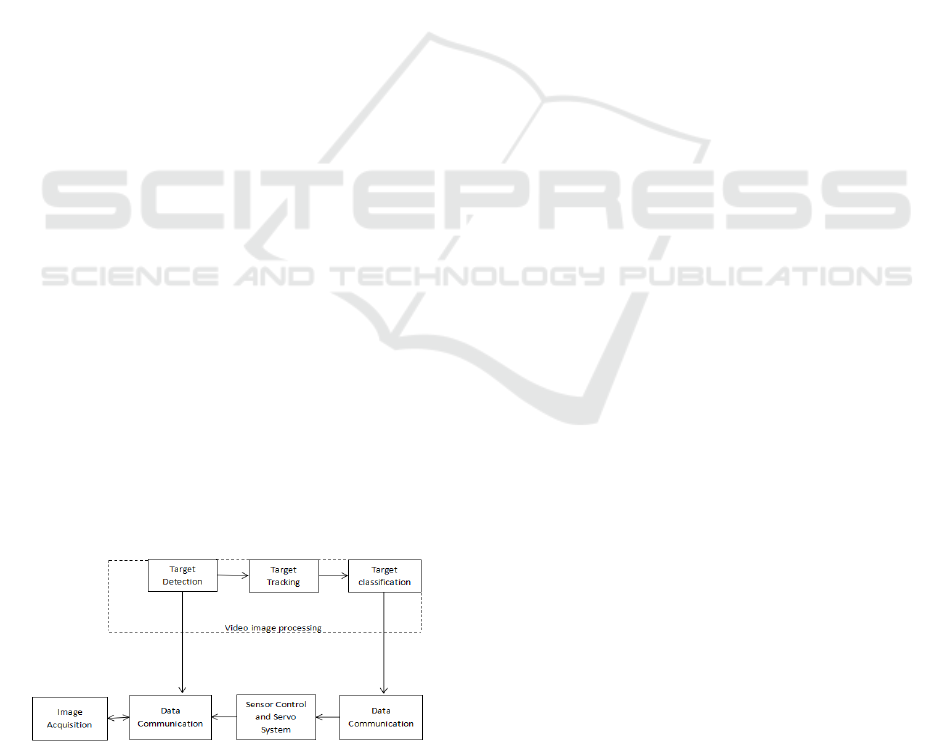
system that is formed is shown in Figure 1.1. The
shipping monitoring system collects images or video
and transmits it to image processing equipment,
detecting targets according to ship template
matching, and Track your goals.
Figure 1.1 Block Diagram of Ship Automatic Tracking
System.
In this paper, the sports ship is taken as the
tracking target, and each frame of image in the video
is taken as the object of processing, and the image is
enhanced. Then, the target ship is tracked by
Kalman and particle filter respectively.
2.ALGORITHM PRINCIPLE
ANALYSIS
2.1 MeanShift Algorithm
Mean Shift is a typical algorithm for the offset
vector. In the target tracking, the probability density
function is used to iteratively search for the target
color feature to track the target. Now commonly
referred to as Mean Shift algorithm belongs to the
search and match category in the tracking.
According to the maximum similarity of the tracking
template, the mean value of the current point and the
mean value of the shifted point are automatically
found in the neighboring area. This is a relatively
simple density estimation model. Constant search
until the calculated offset point is the last pixel to
scan the entire image. [1,2]. The specific process of
the algorithm is as follows:
(1) The target model of the initial frame
In the target search window space, the interval is
divided into K equal intervals, and the central pixel
coordinate of the search window in the initial frame
is set as the coordinate of the i-th pixel in the image
space area. In addition,
(
)
2
xk
is used to represent
the kernel function selected during processing and
the window width is h. Then the probability of the u-
th eigenvalue can be expressed by formula (5.1):
(2.1)
In (2.1), the membership of the color
corresponding to the characteristic value u in the
coordinates can be judged by b and, in the color
space, C as the constant coefficient makes
probability and normalization:
∑
=
=
n
i
q
1
1
ˆ
(2.2)
(2)Current frame model
According to the establishment of the initial
frame model, the probability of the u-th feature
value of the search window in the current frame can
also be expressed as:
(2.3)
In equation (2.3), the central pixel coordinates
corresponding to the current frame search window in
the initial frame model correspond to C in equation
(2.1).
(2)Similarity function
The similarity between the target model and the
current frame model in the initial frame can be
described by a similarity function, which is defined
as Equation (2.4):
(2.4)
among them
In the feature interval, the desired MeanShift
vector can be obtained when the similarity function
ρ(y) is at the maximum value[3]:
.
(2.5)
2.2Particle Filter Fundamentals
The basic idea of particle filtering is to first generate
a set of random samples in the state space based on
the empirical conditional distribution of the system
state vectors. These samples are called particles, and
then the weights and positions of the particles are
continuously adjusted according to the
measurements, and the particles are adjusted. The
information corrects the initial distribution of
experience conditions. The essence of this approach
is to approximate the associated probability
distributions using discrete random measures
consisting of particles and their weights, and
recursively update the discrete random densities
according to the algorithm. When the sample size is
large, this Monte Carlo description approximates the
true nonlinear stochastic system of the state variable,
and the precision can be approximated to the optimal
estimate. It is a very effective nonlinear filtering
technique [4].
Particle filtering, also known as sequential
Monte Carlo method (SMC), refers to finding a
series of random samples that can approximately
express the probability density function
()
kk
zxp |
in the state space, and replacing the integral
operation with an arithmetic mean value to obtain
the state minimum variance The process of
estimation. These random samples are called
"particles."
The particle filter algorithm is as follows:
Combining the SIS with the particle resampling
method, a complete particle filter algorithm can be
obtained. Specific steps are as follows:
1) Initialization
Based on the distribution, random sampling in
the vicinity to obtain a series of particles
2)SIS
Usually the importance
distribution
()
kkk
zxxq
:11:0
,|
−
can be simplified to
sample N particles accordingly
()
1
|
−
∝
kk
i
k
xxpx
3) Calculate weights
Calculate the weight of each particle
()
i
k
w
and
normalize it
() () ()
∑
=
=
N
i
i
k
i
k
i
k
www
1
/
.
4) A posteriori probability estimate
Output a set of weighted
particles
(){}
Niwx
i
k
i
k
,...,2,1,, =
, according to the
weighted average or maximum posterior probability
[]
)(
ˆ
1
0
uxb
h
xx
kCq
i
n
i
i
−
⎟
⎟
⎠
⎞
⎜
⎜
⎝
⎛
−
=
∑
=
δ
()
[]
∑
=
−
⎟
⎟
⎠
⎞
⎜
⎜
⎝
⎛
−
=
n
i
i
i
h
uxb
h
xy
kCyp
1
0
0
)(
ˆ
δ
()() ()
∑∑
==
⎟
⎟
⎠
⎞
⎜
⎜
⎝
⎛
−
+=
h
n
i
i
i
h
m
u
uu
h
xy
kw
C
qypqy
1
2
1
2
ˆˆ
2
1
ˆ
,
ˆ
ρρ
()
()
[]
∑
=
−=
m
i
i
n
u
i
uxb
yp
q
w
1
0
ˆ
ˆ
δ
()
0
1
2
0
1
2
01,
ˆ
ˆ
y
h
xiy
gw
h
xy
gwx
yyym
h
h
n
i
i
n
i
i
ii
Gh
−
⎥
⎥
⎥
⎥
⎥
⎦
⎤
⎢
⎢
⎢
⎢
⎢
⎣
⎡
⎟
⎟
⎠
⎞
⎜
⎜
⎝
⎛
−
⎟
⎟
⎠
⎞
⎜
⎜
⎝
⎛
−
=−=
∑
∑
=
=
of the particle, to obtain the posterior probability
estimate of the current time k.
5) Particle resampling
According to the particle weights, the sample set
is re-sampled, the large-weighted particles are
divided into multiple particles, the small-weighted
particles are deleted, and the new N particles are
obtained.
6) State transfer
When k+1 arrives, record the observations and
repeat from 2 to 6.
3. SPORTS SHIP TRACKING
EXPERIMENT
3.1 Mean Shift Tracking Algorithm
The traditional Mean Shift algorithm was used for
target tracking in the experiment. The first is the
initialization of the target tracking, which can be
used to obtain the circumscribed rectangle of the
initial target that needs to be tracked. However, the
main research focus of this paper is to track the
algorithm and not focus on the target detection
module, so the manual selection method is selected
by the mouse. Then calculate the histogram
distribution of the search window weighted by the
kernel function, and use the same method to
calculate the histogram distribution of the
corresponding window of the Nth frame; use the
principle of maximum similarity of the distribution
of the two target templates to maximize the search
window along the density increase. Move in the
direction to get the true position of the target. The
tracking steps are as follows:
1) Calculate the probability density of the target
template, the target estimated position and the
nuclear window width h;
2) Using the target position of the initial frame to
calculate the candidate target template;
3) Calculate the weight value of each point in the
current window;
4) Calculate the new position of the target
(3.1)
The Mean Shift algorithm continuously iterates
and finally finds the optimal position of the target in
the image sequence.
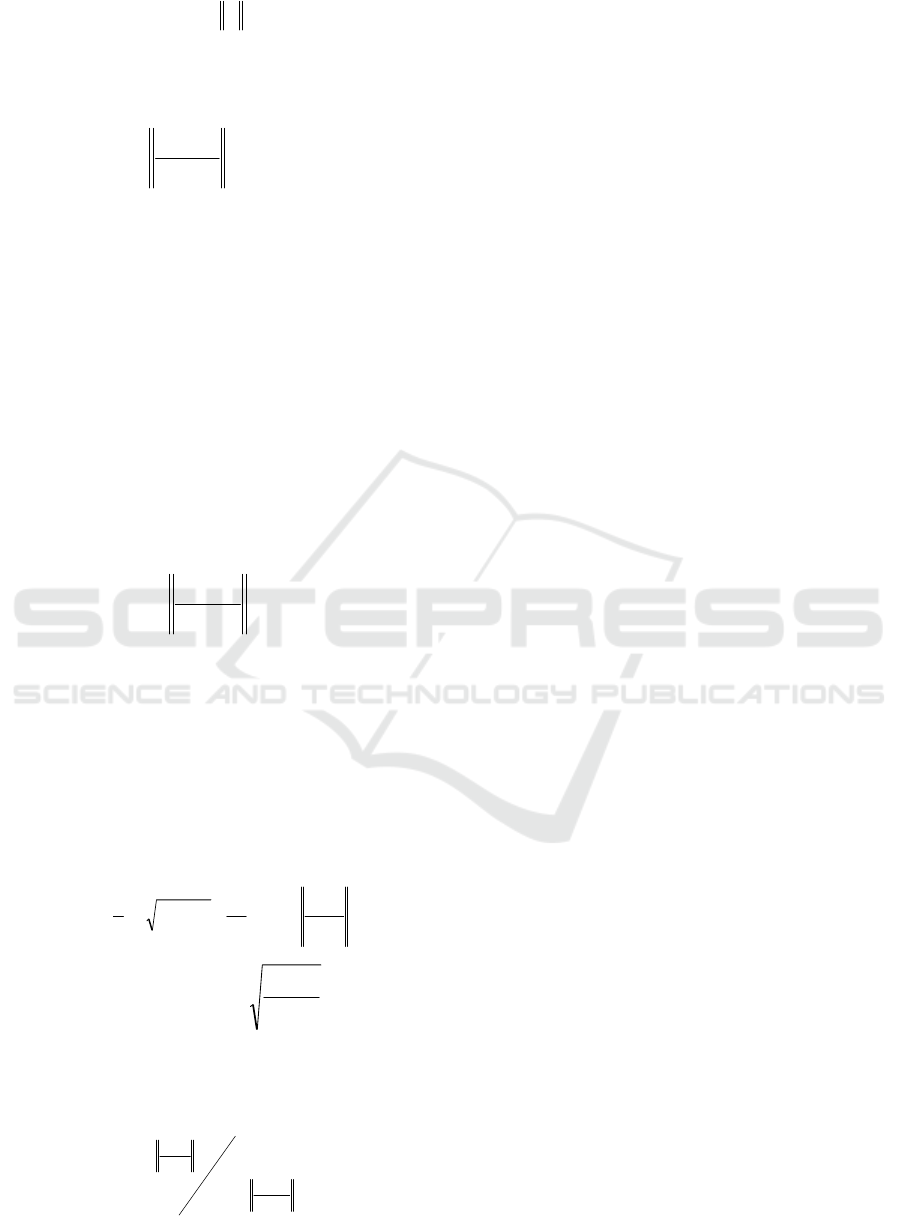
In the experiment, the tracking window is first
determined, the tracking target model of the initial
frame is set, the target to be tracked is selected in the
first frame, and a rectangle, that is, the ship feature
search window containing the ship's target is framed,
also called the tracked target area, and cut This area
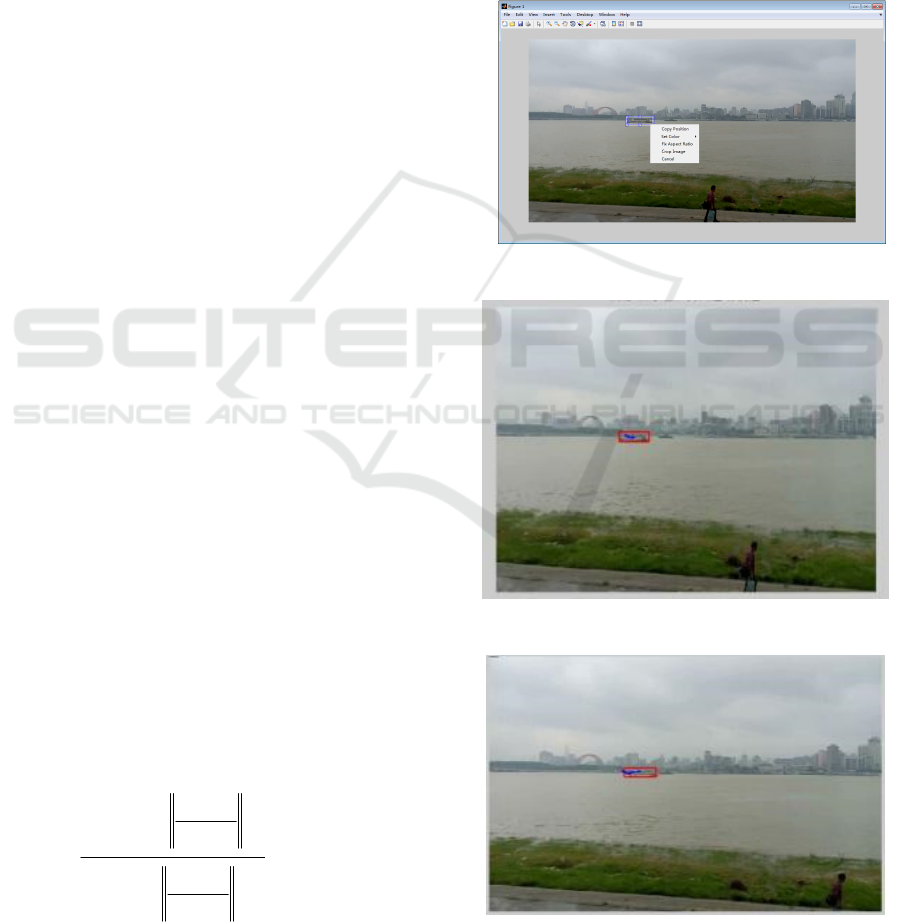
is shown in Figure 3.1. After the end of the tracking,
observe the record tracking results, as shown in
Figures 3.2 to 3.5.
Figure 3.1 Image Selection.
Figure 3.2 Frame 20.
Figure 3.3 Frame 50.
∑
∑
=
=
⎟
⎟
⎠
⎞
⎜
⎜
⎝
⎛
−
⎟
⎟
⎠
⎞
⎜
⎜
⎝
⎛
−
=
m
i
i
i
m
i
i
ii
h
xy
gw
h
xy
gwx
y
1
2
0
1
2
0
1
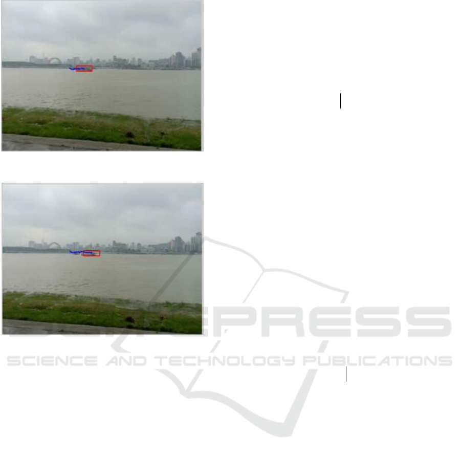
Figure 3.4Frame 70.
Figure 3.5 Frame 100.
From the experimental results, it can be seen that the
two ships are staggered at the 50 frames, but the
tracking frame is slightly shifted at a video around
the middle 100th frame, but after that, the tracking
frame is restored accurately until the final 273th
frame. Observe the tracking trajectory is basically in
line with the movement, but the occurrence of up
and down jump, on the one hand, there is tracking
error, but the main reason is that there is no use of a
tripod in the video capture process, the image jitter,
it is acceptable error range.
3.2 Ship Tracking Based on Particle
Filter
Particles used in target tracking usually refer to
target status information, including target position,
size, color, and motion information. The specific
implementation steps are as follows [5]:
1) Initialization
The initial position of the target
0
X
is selected
and N particles are randomly distributed near
0
X
.
2) Get particle weight
Assuming the system is in a state such as
n
XXX ,...,
21
, Any
i
X , i = 1, 2, ..., n, we call a
particle that represents a particle-centric image
block. Each particle's position, color, edge, and
other information together form the current state of
the moment. Z is the observed value of the system at
this time, and
)(
:1 kk
xzp
is obtained based on
historical information. To estimate the exact position
of the target X, it is necessary to operate on the
particles. Each particle
i
X corresponds to a
rectangular frame, and the color in the frame is
counted to obtain a 16-dimensional color histogram
vector
i
H
. Each color histogram has 16 bins
containing 16 grayscale values (0~255/16). After the
statistics are finished, The
i
H is normalized so that
the sum of the squares of each bin is 1, which is a
16-dimensional unit vector.
The weight
i
W of each
i
H can be understood
as the inner product of the color histograms
H
and
i
H of the target template, that is, the quantities of
each bin are multiplied and added. This represents
the similarity between the image region represented
by the current particle and the target template. The
higher the weight, the more similar the particle is to
the target. The
n
XXX ,...,
21
weight
n
WWW ,...,
21
calculated from
)(
:1 kk
xzp
, where ><
i
HH ,
represents the inner product operation.
3) Predict the current position
From the weighted average of the obtained
particles
n
XXX ,...,
21
and the corresponding
weight
n
WWW ,...,
21
, the system state can be
estimated:
nn
WXWXWXX *...**
2211
+++= , where
i
X represents the location information of the center
of the area. The resulting X is approximately equal
to the posterior probability estimate and predicts the
current position of the target.
4) Particle resampling
As the number of tilts of the video increases, the
weights will become more and more concentrated on
a small number of particles. Most of the other
particles have very small weights. Before entering
the next iteration, the particle weights are
redistributed to make them all the same. Therefore,
the particles need to be re-sampled, ie, N particles

n
XXX
′′′
,...,
21
are regenerated. The regenerated
particles all come from the original particle set
n
XXX ,...,
21
, in which the large particles
generated by the weights generate more new
particles, and the particles having the smaller
weights correspond to fewer new particles.
5) State transfer
At the next moment, the particles are updated,
that is,
i
X
′
becomes
i
X
′′
. Since the probability that
the state transition from
i
X
′
to
i
X
′′
can be obtained
from the state matrix is
)(
1−kk
xxp
, the probability
of changing from
i
X
′
to
i
X
′′
is equal to
)(
1−kk
xxp
.
6) Repeat 2 to 5.
In the experiment, the number of particles was
selected as 200. The particle filter algorithm of this
paper also adopts the method of manually selecting
the tracking target. First, the initial frame is
displayed, and a rectangle, that is, the ship feature
search window containing the ship's target is
selected by using the selection box, and the ship's
edge is cut as far as possible, and right-cut. Use the
[temp,rect]=imcrop(I) format to cut, the image
matrix of the ship model is saved in the temp
variable, and then a histogram is calculated for the
variable; the initial position coordinates of the ship
are stored in the rect variable for calculation The
center coordinates of the ship.
3.3 Error Analysis
In this paper, the distance between the tracking
center point and the actual movement center point is
calculated to calculate the error of comparing the
two algorithms. The center point of the actual
movement uses the manual selection method, writes
a program, selects 9 frames, and determines the
coordinates of the center point; then uses a
polynomial fitting method to perform 6 fittings to fit
the actual motion trajectory; then it calculates the
two tracks separately. The error between the curve
and the trajectory is measured by the error and
variance of the average per frame. The error
calculation result shows the MATLAB running
screenshot, as shown in Table 1.
Table 1 Comparison of tracking errors.
Average per frame error (pixels) Average gap between two
algorithms per frame (pixels)
Particle filter method 3.7212 5.7782
Mean shift method 2.3213
From the above tracking results, it can be seen
that both algorithms have jitter in the tracking
process, but the overall trend is correct, and the
mean error using the mean shift method is smaller
than the particle filter method, and the difference
between the two methods does not exceed 6 pixels.
3.4 Real-time Analysis
Use the tic and toc commands to output the total
running time of the program. The results are shown
in Table 2.
Table 2 Runtime Comparison.
Tracking algorithm Running time (s)
Particle filter algorithm 48.151951
Mean shift algorithm 115.003216
It can be seen that the operation time of the
particle filter algorithm is far less than the mean shift
algorithm, and the real-time performance is better.
This aspect is the reason for the algorithm, and on
the other hand, it is the reason for the design of the
program itself.
3.5 Effect of Particle Number on Particle
Filtering Tracking
Set the number of particles to 100, 200, 500, 1000,
and 2000, and observe the effect on the program.

The change in the running time is shown in Table 3. The error is shown in Table 4.
Table 3 Effect of Particle Number on Running Time.
Number of particles Running time (s)
100 35.889891
200 48.151951
500 63.085486
1000 121.126432
2000 196.054916
Table 4 Effect of Particle Number on Tracking Error.
Number of particles Average per frame error (pixels)
100 3.9718
200 3.7212
500 3.0853
1000 2.7546
2000 2.3691
It can be seen that the number of particles
increases, the amount of calculation increases, the
running time of the program becomes longer, and
the real-time performance becomes worse; the
tracking effect seems to be better intuitively, but the
actual error change is not obvious, which is related
to the number of times of polynomial fitting, Select
manually when the target is selected. The initial
template is inconsistent.
4 CONCLUSIONS
The tracking accuracy and real-time performance of
the two algorithms are compared. It is found that the
accuracy of the particle filter tracking algorithm is
lower than that of the mean-shift algorithm, but the
real-time performance is better. Afterwards, the
effect of particle number on particle filtering was
studied. It was found that as the number of particles
increases, the tracking accuracy increases, but the
running time becomes longer and the real-time
performance becomes worse
.
REFERENCES
1. Zhu shengli. Study on MeanShift and related
algorithm in video tracking [D]. Hangzhou: zhejiang
university,2007
2. Cheng Yi Zong.MeanShift,Mode Seeking,and
Clustering[J].IEEE transactions on pattern analysis
and machine intelligence,1995,8,17(8):790-798
3. Collins Robert T.MeanShift blob tracking through
scale space[J].IEEE Computer Society Conference
on Computer Vision and pattern
Recognition,2003,2:234-240
4. Zhu zhiyu. Particle filtering algorithm and its
application [M]. Beijing: science press, 2010:27-28
5. Hans R. Künsch.Particle filters[J].Statistics,2013
