
Implementation of Fractional Logistic Growth Model in Describing
Rooster Growth
Windarto, Eridani and Utami Dyah Purwati
Department of Mathematics, Faculty of Science and Technology, Universitas Airlangga, Surabaya, Indonesia
Keywords: fractional order, logistic growth model, particle swarm optimization method, rooster growth.
Abstract: Fractional order calculus was used in the study of viscoelastic medium (a medium with viscosity and elasticity
properties), image signal processing, and population growth modeling. In this paper, the fractional order of
logistic growth model was used to describe the dynamic growth of rooster, by which the rooster growth data
was cited from the literature. We also used the particle swarm optimization method to estimate parameters in
the fractional order logistic model. We found that the fractional order model is more accurate than the classical
logistic growth model in describing the rooster growth.
1 INTRODUCTION
Logistic growth model is widely used to describe a
life organism growth. The logistic growth of a single
species is governed by the following differential
equation.
(1)
Here represents the number of population of the
species at time and correspond to per capita
growth rate and carrying capacity respectively. If the
initial value
is positive, then analytical solution of
the logistic growth model in Eq. (1) given by Aggrey
(2002) and Windarto et al. (2014) is as follows.
(2)
where
The logistic growth ordinary differential equation
in Equation (1) has been generalized into the
fractional order logistic differential equation given by
El-Sayed et al. (2007).
(3)
Here, is fractional order where For
any positive initial value
, the exact solution of
fractional order logistic differential equations cannot
be determined. In this situation, heuristic method such
as simulated annealing, genetic algorithm and particle
swarm optimization method can
be applied to
estimate parameter values from the fractional order
logistic differential equation.
Particle swarm optimization is an optimization
method based on a population-based stochastic
(probabilistic) search process (Eberhart R. &
Kennedy, 1995; Kuo et al., 2011). Particle swarm
optimization method has been widely applied in many
areas, including performance improvement of
Artificial Neural Network (Salerno, 1997; Zhang et
al., 2000), scheduling problems (Koay and
Srinivasan, 2003; Weijun et al., 2004), traveling
salesman problems (Wang et al, 2003), vehicle
routing problems (Wu et al., 2004) and clustering
analysis (Kuo et al., 2011).
In this paper, particle swarm optimization method
was applied for predicting the parameters in fractional
logistic growth model. The remainder of this paper is
organized as follows. Section 2 briefly presents
particle swarm optimization method. Section 3
presents the implementation of fractional logistic
growth model for describing poultry growth. In
addition, parameters in the fractional logistic growth
was estimated by using particle swarm optimization
method. Finally, conclusions are presented in Section
4.
Windarto, ., Eridani, . and Purwati, U.
Implementation of Fractional Logistic Growth Model in Describing Rooster Growth.
DOI: 10.5220/0007547505830586
In Proceedings of the 2nd International Conference Postgraduate School (ICPS 2018), pages 583-586
ISBN: 978-989-758-348-3
Copyright
c
2018 by SCITEPRESS – Science and Technology Publications, Lda. All rights reserved
583
2 PARTICLE SWARM
OPTIMIZATION METHOD
Particle swarm optimization algorithm was invented
by Eberhart and Kennedy in 1995. The algorithm has
similarities with evolutionary computation methods
such as genetic algorithm. The particle swarm
optimization algorithm is initialized with a population
of random solutions and searches optimal solution
updating generations. However, particle swarm
optimization algorithm does not have crossovers and
mutation operators. Potential particles (solutions) in
the particle swarm optimization algorithm move
through the solution space by following the current
optimum particles (Kuo et al., 2011).
The particle swarm optimization algorithm starts
by randomly choosing initial (particles) solutions
within the search space. Fitness function of the
current position of every particle is evaluated. If the
fitness value is better than the previous best value,
then the local best position of a particle is updated.
The global best is updated based on the best fitness
value found by any of the neighbour.
The particle swarm optimization algorithm
consists of the following steps, which are repeated
until some termination conditions are met (Kuo et al.,
2011; Rini et al., 2011):
1. Evaluate the fitness of every particle (solution).
For a maximization problem, the greater the
objective function, the greater of the fitness will
be. On the other hand, for a minimization
problem, the smaller the objective function, the
greater the fitness will be.
2. Update particle best (local best) position and
global best position.
3. Update velocity of every particle using the
following equation
(4)
where
and
are the velocity of particle
and position of particle at discrete time t,
and
are the local best and
global best position at time t,
and
are
uniformly distributed random number between
zero and one.
4. Update position of every particle using the
following equation
(5)
In Equation (4), is the inertia weight, whereas
and
are cognitive coefficient and social
coefficient respectively. The value of the inertial
coefficient is typically between 0.8 and 1.2, while the
values of cognitive coefficient and social coefficient
are typically close to 2.
In order to prevent the particles from moving very
far beyond the search space, velocity clamping
technique can be applied to limit the maximum
velocity of every particle. For a search space
bounded by the range
, the velocity is
limited within the range
where
for some constant
Some common stopping conditions in particle
swarm optimization include a predetermined number
of iterations, a number of iterations since the last
update of global best solution, or a pre-set target
fitness value (Kuo et al., 2011; Rini et al., 2011).
3 IMPLEMENTATION OF
FRACTIONAL LOGISTIC
GROWTH MODEL
In this section, the fractional order logistic growth in
Equation (3) for describing rooster growth was
applied. Parameters in the model were estimated from
some rooster weight data cited from the literature.
The rooster weight data
at the day
are
presented in the Table 1 (Aggrey, 2002; Windarto et
al., 2014).
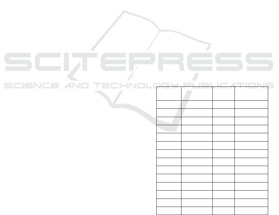
Table 1: Means of the rooster weight data (y).
t
(days)
y (grams)
t
(days)
y (grams)
0
37
42
519.72
3
41.74
45
577.27
6
59.19
48
633.59
9
79.94
51
667.18
12
102.96
54
717.17
15
132.13
57
786.35
18
170.18
71
1069.28
21
206.56
85
1326.49
24
250.71
99
1589.71
27
285.27
113
1859.26
30
324.92
127
2015.44
33
372.83
141
2142.31
36
417.41
155
2220.54
39
469.13
170
2262.63
From Table 1, we found that initial weight of the
rooster is
grams. Parameters (the
fractional order), (the rooster growth rate) and
(carrying capacity parameter or mature weight of the
ICPS 2018 - 2nd International Conference Postgraduate School
584
rooster) were estimated. Particle swarm optimization
method was applied and described in the Section 2
with the inertia weight parameter the
cognitive coefficient parameter
and the social
coefficient parameter
respectively. The
particle swarm optimization algorithm was
implemented until 100 iterations.
Parameters in the fractional order logistic growth
model were estimated such that the
minimum mean square error (MSE) given by
(6)
Here,
and
are rooster weight data and predicted
rooster weight at the i-th day, while n is the number
of observation data. The estimation results of
fractional order logistic growth are presented in Table
2.
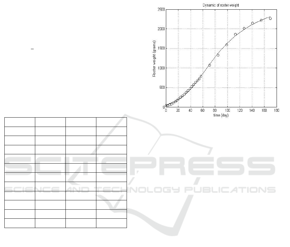
Table 2: The estimated parameters using particle swarm
optimization method.
r
K
MSE
0.3999
0.3018
4000.00
714.93
0.4753
0.2461
3491.86
772.41
0.5242
0.2182
3152.67
1001.66
0.4080
0.2946
3898.96
872.93
0.4620
0.2524
3529.82
1248.19
0.4678
0.2500
3565.34
807.87
0.4722
0.2466
3500.00
803.93
0.4395
0.2738
3630.19
710.35
0.4695
0.2500
3500.00
680.08
0.3621
0.3319
4500.00
996.41
0.4705
0.2498
3500.00
711.06
It was found from Table 2 that the best parameters
were where
the mean square error 8. Meanwhile,
the best parameters for logistic growth model were
where the
mean square error . Hence, we found
that the fractional order logistic model was more
accurate than the (classical) logistic growth model.
It was known that the analytical solution of the
fractional order logistic growth model converged to
the carrying capacity parameter or the mature weight
parameter (K). Here, asymptotic rooster weight (y(t))
tended to the mature weight parameter. Dynamic of
the rooster weight for the best parameters also
confirmed the analytical properties. The rooster
weight also tended to the mature weight parameter. A
comparison
between observed and predicted rooster
weight is
shown in Figure 1. From the figure, it can
be seen that the predicted rooster weight of the
fractional order logistic model did not significantly
differ from the observed data.
Figure 1: Comparison between observed and predicted
rooster weight.
4 CONCLUSION
Fractional order growth model has been applied to
describe dynamic of rooster weight. Parameters of the
model were estimated from secondary data cited from
literature. The fractional order logistic model was
found to give more accurate results than the classical
logistic growth model.
ACKNOWLEDGEMENTS
A part of this research was supported by the Ministry
of Research, Technology and Higher Education, the
Republic of Indonesia through PUPT project.
REFERENCES
Aggrey, S.E., 2002. Comparison of Three Nonlinear and
Spline Regression Models for Describing Chicken
Growth Curves, Poultry Science 81:1782-1788, 2002.
Eberhart R. & Kennedy, J., 1995. A new optimizer using
particle swarm theory, Proceedings of the Sixth
International Symposium on Micro Machine and
Human Science, 39–43.
El-Sayed, A.M.A., El-Mesiry, A.E.M. & El-Saka, H.A.A.,
2007. On the fractional-order logistic equation,
Applied Mathematics Letters 20, 817–823.
Implementation of Fractional Logistic Growth Model in Describing Rooster Growth
585

Koay, C.A. & Srinivasan, D., 2003, Particle swarm
optimization-based approach for generator
maintenance scheduling. In: Proceedings of the 2003
IEEE swarm intelligence symposium, 167–173.
Kuo, R. J., Wang, M. J. & Huang, T. W., 2011. An
application of particle swarm optimization algorithm
to clustering analysis, Soft Computing 15, 533–542.
Rini, D.P., Shamsuddin, S.M., Yuhaniz, S.S., 2011. Particle
Swarm Optimization: Technique, System and
Challenges, International Journal of Computer
Applications Vol. 14 No.1.
Salerno, J., 1997. Using the particle swarm optimization
technique to train a recurrent neural model,
Proceedings of the Ninth IEEE International
Conference on Tools with Artificial Intelligence, 45–
49.
Weijun, X., Zhiming, W., Wei, Z. & Genke, Y., 2004. A
new hybrid optimization algorithm for the job-shop
scheduling problem, Proceedings of the 2004
American Control Conference, 5552–5557.
Wang, K.P., Huang, L., Zhou, C.G. & Pang, W., 2003.
Particle swarm optimization for traveling salesman
problem, 2003 International Conference on Machine
Learning and Cybernetics, 1583–1585.
Windarto, Indratno, S. W., Nuraini, N., & Soewono, E.,
2014. A comparison of binary and continuous genetic
algorithm in parameter estimation of a logistic growth
model, AIP Conference Proceedings 1587, 139–142.
Wu, B., Yanwei, Z., Yaliang, M., Hongzhao, D. & Weian,
W., 2004. Particle swarm optimization method for
vehicle routing problem, Fifth World Congress on
Intelligent Control and Automation, 2219–2221.
Zhang, C., Shao, H. & Li, Y., 2000. Particle swarm
optimization for evolving artificial neural network,
IEEE international conference on systems, man and
cybernetics, 2487–2490.
ICPS 2018 - 2nd International Conference Postgraduate School
586
