Geographically Weighted Regression for Prediction of

Underdeveloped Regions in East Java Province Based on Poverty

Indicators

Rusdi Hidayat N

, Bambang Widjanarko Otok

, Zumarsiyah Mahsyari

, Siti Halimah Sa’diyah

, and

Dimas Achmad Fadhila

Business Administration Study Program, FISIP, UPN “Veteran” East Java, Surabaya

Department of Statistics, FMKSD, Institut Teknologi Sepuluh Nopember, Surabaya

Keywords: GWR, Kernel Function, Adaptive Bisquare, Underdeveloped Regions, Poverty.

Abstract: Underdevelopment problem of a region can be seen from the dimensions of the economy, human resources,

financial capability, infrastructure, accessibility, and regional characteristics. One method to see a region is

underdeveloped or not is by looking the percentage of people living in poverty in a region in the publication

data of underdeveloped regional indicators issued by the Central Bureau of Statistics (BPS). The results

showed that the percentage of people in East Java Province who are living in poverty using linear regression

is not yet appropriate. The percentage of people living in poverty spread spatially because there is

heterogeneity between the observation sites which means that the observation of a location depends on the

observation in another location with adjacent distance so that the spatial regression modeling was done with

Adaptive Bisquare Kernel function. The grouping results with GWR resulted in nine groups based on

significant variables. Each group eas characterized by life expectancy, mean years of schooling, expenditure

and literacy rate.

1 INTRODUCTION

Underdeveloped regions are an area with districts

where communities and their territories are

relatively less developed than other regions on a

national scale. The backwardness of the area can be

measured based on six main criteria: economy,

human resources, infrastructure, regional financial

capacity, accessibility and regional characteristics

(Directorate General of Underdeveloped Regions

Development, 2016). To identify whether a district

is underdeveloped can be measured using

predetermined standards referring to the Minister of

Village Regulations, Development of

Underdeveloped Regions and Transmigration No. 3

of 2016 on Technical Guidelines for the

Determination of Indicators of Underdeveloped

Regions Nationally. The purpose of this paper is to

identify the problem of backwardness of a region

based on the percentage of poor people indicator.

If a study is influenced by the spatial aspect, then

it is necessary to consider spatial data on the model.

Spatial data is data that contains location

information. In spatial data, frequent observations at

a site depends on observation in another adjacent

location (neighboring) (Anselin, 1988). The law is

the basis for reviewing problems based on the

effects of location or spatial methods. In modeling,

if the classical regression model is used as an

analytical tool on spatial data, it can lead to

inaccurate conclusions because the assumption of

error is mutually free and the assumption of

homogeneity is not met.

2 LITERATURE RIVIEW

Geographically Weighted Regression (GWR) model

is the development of a regression model where each

parameter is calculated at each observation location,

so that each location of observation has different

regression parameter values. The GWR model is an

expansion of the global regression model in which

the basic idea is derived from non-parametric

regression (May, 2006). The y response variable in

the GWR model is predicted by the predictor

898

Hidayat N, R., Otok, B., Mahsyari, Z., Saâ

Zdiyah, S. and Fadhila, D.

Geographically Weighted Regression for Prediction of Underdeveloped Regions in East Java Province Based on Poverty Indicators.

DOI: 10.5220/0007553708980907

In Proceedings of the 2nd International Conference Postgraduate School (ICPS 2018), pages 898-907

ISBN: 978-989-758-348-3

variable and each regression coefficient depends on

the location where the data is observed. The GWR

model is stated as follows (Fotheringham et al.,

2002):

() ()

iii kiiiki

yuv uvx

ββ

=+ +

∑

(1)

Estimation of GWR model parameters is done by

Weighted Least Squares (WLS) method through

assigning different weights to each location where

data is observed. Suppose weighting for each

location

()

jii

wuv

, j = 1, 2,…,n then the

parameters at the observation location

()

vu ,

then

the parameters at the observation location

()

jii

wuv

in equation (1) and then minimize the sum of

residual squares, or in the matrix form the sum of the

residual squares is:

() () () ()

() ()()

,,2,,

, , ,

TT TT

ii ii ii ii

ii ii ii

uv uv uv uv

uv uv uv

=−

ε W ε yW y β XW y

β XW Xβ

(2)

with:

()

pii

⎛⎞

⎜⎟

⎝⎠

and

() ()() ()

()

,diag ,, ,,, ,

ii ii ii n ii

uv wuv w uv w uv=W L

If equation (2) is lowered to

()

uvβ

and the

result is equal to zero then obtained parameter

estimator GWR model:

() () ()

,, ,

ii ii ii

uv uv uv

−

⎡⎤

⎣⎦

β XW X XW y

(3)

For instance

()

1, , , ,

iiiip

xx=x L

is the i row

element of the X matrix. Then the prediction value

for y at the observation location

()

can be

obtained in the following way:

() ()

()

,,,

TTT T

iiii i ii ii

yuv uv uv

−

==x β xXW X XW y

So for all observations can be written as follows:

()

ˆˆˆ ˆ

,,,

yy y==yLyL

and

()()

ˆˆ ˆ

,,,

εε ε

==ε I-L

with I is an identity matrix of nxn and

()

111 11

222 22

TT T

nnn nn

uv uv

−

⎛⎞

⎜⎟

⎝⎠

xXW X XW

(4)

The weighting role of the GWR model is

important because this weighted value represents the

location of the observed data with each other. The

weighting scheme on GWR can use several different

methods. There is some literature that can be used to

determine the weighting for each different location

on the GWR model, such as by using Kernel

Function.

The Kernel Function is used to estimate the

parameters in the GWR model if the distance

function

(

)

is a continuous and monotonous

function down (Chasco, Garcia and Vicens, 2007).

Weights that are formed by using this kernel

function are the Gaussian Distance Function,

Exponential Function, Bisquare Function, and

Tricube Kernel Function and involve the smoothing

parameter (Lesage, 2001). Cross Validation (CV)

method to select the optimum bandwidth, which is

mathematically defined as follows:

()

CV h y y h

≠

=−

∑

with

()

≠

)

is the value of the appraiser

y where

the observations are on location

()

removed

from the estimation process. To get the value

the

optimal is then obtained from

which results in a

minimum CV value.

Hypothesis testing on the GWR model consists

of testing the suitability of the GWR model and

testing the model parameters. Testing the suitability

of the GWR model (goodness of fit) is done with the

following hypothesis:

()

H: ,

kii k

ββ

(there is no significant

difference between global regression model

and GWR)

H :

At least, there is one

()

kii k

ββ

≠

for each

0,1, 2, , , and 1, 2, ,kpin==LL

(there is a significant difference between the

global regression model and GWR).

Determination of test statistics based on Residual

Sum of Square (RSS) obtained respectively below

Geographically Weighted Regression for Prediction of Underdeveloped Regions in East Java Province Based on Poverty Indicators

899

dan H

. Under conditions H

, using OLS method

obtained the following RSS value:

() ()()( )

ˆˆ ˆ ˆ

RSS H

==− −= −εε yy yy y IHy

wit

()

−

HXXX X which is idempotent. Under

conditions H

, spatially varying regression

coefficients in equation (1) is determined by the

GWR method, to obtain the following RSS values:

() ()()

()()

ˆˆ ˆ ˆ

RSS H

==− −

=− −

εε yy yy

yIL ILy

(5)

so obtained the following test statistic (Leung et al.,

2000a):

()

RSS

RSS n p

⎛⎞

⎜⎟

⎝⎠

−−

Below H

will follow the F distribution with

degrees of freedom

⎛⎞

⎜⎟

⎝⎠

and

()

1df n p=−−

. If taken the level of significance

then reject H

11,,df df

−

with:

()()

, 1, 2

tr i

⎛⎞

⎡⎤

=−− =

⎜⎟

⎢⎥

⎣⎦

⎝⎠

IL IL

. (6)

Another alternative as a test statistic is to use the

difference in the number of residual squares below

and below H

(Leung et al., 2000a), i.e:

() ()

()

()()()

()()

011

RSSH RSSH

RSS H

−

⎡⎤

−−− −

⎣⎦

−−

yIH ILILy

yIL ILy

Below H

will follow the distribution F with

degrees of freedom

and

⎛⎞

⎜⎟

⎝⎠

. If

taken the level of significance

then reject H

2,,df df

≥

with:

( )()()

, 1, 2

tr i

⎛⎞

⎡⎤

=−−−− =

⎜⎟

⎢⎥

⎣⎦

⎝⎠

IH IL IL

If it is concluded that the GWR model is

significantly different from the global regression

model, then the next step is to perform a partial test

to find out whether there is a significant influence

difference from the predictor variable

between

one location and another (May, He and Fang, 2004).

This test can be done by hypothesis:

() ( ) ( )

11 2 2

,, ,

kk knn

uv u v u v

ββ β

===L

(there

is no significant difference of influence from the

predictor variable

between one location and

another)

: At least, there is one,

()

, , for 1, 2,...,

kii

uv i n

()

0,1, 2, ,kp= L

which

different. (there is a significant effect difference

from the predictor variable

between one location

and another location).

To perform the above test it is determined first

variance

()

iik

vu ,

(i = 1, 2, ..., n) which denoted

by:

() ()

ˆˆ

kkiikii

Vuvuv

ββ

⎛⎞

=−

⎜⎟

⎝⎠

⎡⎤

=−

⎢⎥

⎣⎦

∑∑

β IJβ

with

()

kii

knn

⎛⎞

⎜⎟

⎝⎠

While the test statistic used is:

RSS(H )

kk k

Vtr

⎛⎞

⎡⎤

−

⎜⎟

⎢⎥

⎣⎦

⎝⎠

BI JB

with:

() ()

11 11

22 22

TT T

knn nn

uv uv

−

⎛⎞

⎡⎤

⎣⎦

⎜⎟

⎡⎤

⎜⎟

⎣⎦

⎜⎟

⎡⎤

⎣⎦

⎝⎠

eXW X XW

is column vector which is size

()

1p +

which is

worth one for the k elements for the other. Matrix

as in (4) and RSS (H

) as in the equation (5).

ICPS 2018 - 2nd International Conference Postgraduate School

900

Below H

, test statistic

will be distributed F

with degrees of freedom

⎛⎞

⎜⎟

⎝⎠

and

⎛⎞

⎜⎟

⎝⎠

with

ik k

⎛⎞

⎡⎤

=−

⎜⎟

⎢⎥

⎣⎦

⎝⎠

BI JB

i=1,2 dan

as in equation (6). Reject H

3,,df df

≥

(Leung et al., 2000a).

The testing of the significance of model

parameters at each location is done by partially

testing the parameters. This test is conducted to

determine which parameters significantly affect the

response variable. The form of the hypothesis is as

follows:

()

H: , 0

kii

()

:,0

kii

Huv

≠

with

1, 2, ,kp= L

The parameter estimator

()

uvβ

will follow the

normal multivariate distribution with the average

()

β ,

and the covariance variant matrix

, with:

()

iii ii

uv uv

−

=CXW XXW ,

so it get to:

(,) (,)

kii kii

uv uv

ββ

−

~N(0,1)

with

is the k-diagonal element of the matrix

. So the test statistic used is:

(,)

kii

hit

Below H

T will follow the t distribution with

degrees of freedom

⎛⎞

⎜⎟

⎝⎠

while

is acquired by

rooting

RSS(H )

. If the given level of

significance is

, then the decision to decline H

or in other words parameters

()

kii

significant

to the if model

hit

, where

⎛⎞

⎜⎟

⎝⎠

Akaike Information Criterion Correction (AICc)

method used to select the best model defined as

follows :

()

2ln ln2

2()

ntr

AIC n n n

ntr

σπ

⎧⎫

=++

⎨⎬

−−

⎩⎭

(7)

with :

: The standard deviation estimator value of the

maximum likelihood estimated error, ie

RSS

S : Where projection matrix

=ySy

The best model selection is done by determining the

model with the smallest AICc value (Fotheringham

et al., 2002).

3 METHODOLOGY

This study used secondary data from Publication of

BPS in 2014. The research variables are presented in

Table 1 below.

Table 1: Research variable.

Variable Indicator

Y Percentage of poor people

X1 Life expectancy

X2 Average school duration

X3 Per capita population expenditure

X4 Literacy

Stages performed in the study.

Description of characteristics and pattern of

percentage distribution of poor people in East

Java.

Modeling percentage of poor people in East

Java with Linear Regression and GWR with

AIC criteria. The steps are as follows.

Detection of muticolinearity cases.

ii.

Modeling percentage of poor people in East

Java with Linear Regression:

Calculates the parameter estimator value

of the Linear regression model

Perform parallery testing simultaneously

and partially.

Testing the residual assumption of IIDN.

iii.

Model GWR on the percentage of the poor

in East Java:

Calculate euclidian distance between

observation locations based on

geographical position. Euclidean distance

between location i located at coordinate

, v

) to location j at coordinate (u

)

Geographically Weighted Regression for Prediction of Underdeveloped Regions in East Java Province Based on Poverty Indicators

901

Determine the optimum bandwidth with

CV criteria

Determine the optimum weighting with

the gauss kernel weighted function.

Calculates the value of the GWR model

parameter estimator

Testing GWR parameters (partial test and

partial test)

Comparing the AICc value of the Global / Linear

Regression Model with the GWR model, the

minimum AICc value is the best model.

4 RESULT AND DISCUSSION

The description of this study includes the mean and

standard deviation of each variable which is

presented in Table 2.

Table 2: Description of research variables.

Varia

ble

Minimum Maximum Mean StDev

Y 4.59 25.8 12.1 4.99

X1 62.16 73.3 69.2 3.15

X2 3.49 10.9 7.3 1.72

X3 7143 15492 10013 2062

X4 77.93 98.5 92.3 4.84

4.1 Multicolinearity Detection

One of the requirements in regression analysis with

some predictor variables is that there is no case of

multicollinearity or there is no predictor variable that

has correlation with other predictor variables. The

detection of muticollinearity is based on the

Variance Inflation Factor (VIF) value. Here is the

VIF value of each predictor variable.

Table 3: VIF of predictor variable.

Variabel X1 X2 X3 X4

VIF 2.085 9.066 4.698 4.526

Table 3 shows that all predictor variables have a

VIF value of less than 10. This detects that there are

no multicollinearity cases or no predictor variables

that have correlation with other predictor variables.

4.2 Significance Test of Linear

Regression of Hypertension

Prevalence

Here is the test of the significance of linear

regression parameters either simultaneously or

partially to determine the effect of predictor

variables used. The hypothesis for simultaneous

parameter significance test in linear regression is as

follows.

: β

= β

=…= β

= 0 (parameters have no

significant effect on the mode)

: At least, there is one β

≠ 0; k = 1, 2, …, 4 (at

least, there is one parameter that significantly

affects the model)

Table 4: ANOVA linear regression table.

Variation

Sources

Sum of

Squares

Mean

Square

F P

Regression 598.32 9 66.48 2.14 0.030

Residual 4418.32 142 31.11

Total 5016.64 151

Table 4 yields a value F

count

in the amount of 2,14

and p-value in the amount of 0,030. Based on the

level of significance (

α) in the amount of 5% and

(0,05;9;142)

in the amount of 1,946, obtained decision

reject H

because of value F

count

> F

(0,05;9;142)

or P-

Value < 0,05. This can be interpreted that there is at

least one parameter that has a significant effect on

the prevalence of hypertension.

Furthermore, to determine which predictor

variables that give a significant influence, then the

partial significance of the parameters were tested

and presented in Table 5. The following hypothesis

test of spatial parameter significance of linear

regression model (global)

: β

= 0,

: β

≠ 0, k = 1,2,3,4

Table 5. Parameter test of partial regression coefficients.

Parame-

ter

Coeffi-

cient

Coeffi-

cient

T Sig.

β0 59.720 16.410 3.640 0.001

β1 0.076 0.187 0.410 0.687

β2 -1.422 0.789 -1.800 0.081

β3 -0.000 0.000 -0.140 0.891

β4 -0.454 0.179 -2.530 0.016

ICPS 2018 - 2nd International Conference Postgraduate School

902

Based on the test results in Table 5, with a

significant level (

α) in the amount of 5% and

()

0.025,33

2.035

−−

, it is obtained that all

values of T smaller than t

(0.025,33)

, except parameters

. This shows that the literacy rate variable

significantly affects the percentage of poor people.

4.3 Testing Residual Assumptions

Testing of residual assumptions is identical,

independent, and normally distributed.

4.3.1 Identical Residual Assumption Test

One assumption test in OLS regression is that

residual variance should be homoscedasticity

(identical) or case of heteroscedasticity. How to

identify the case of heteroscedasticity is to create a

regression model between residual and predictor

variables. If there are predictor variables that

significantly affect the model, then it can be said that

the residual is not identical or happened case of

heteroscedasticity. Testing identical residual

assumptions provides information that no cases of

heteroscedasticity or residual have been identical to

a significant level (

α) of 0.05 and

()()

;, 1 0,05;4,33

2.659

pn p

−−

. This is because of

the P-Value (0.119) is bigger than

α (0.05) and F

(1.99) is smaller than 2.659, then there is no

heteroscedasticity.

4.3.2 Independent Residual Assumption

Test

An independent residual assumption test is used to

determine whether or not the relationship exists

between residuals. The test statistic used is Durbin-

Watson. The value of DW = 1.099 earned value

07875,2=d

with

0201,1=

and

9198,1=

. So the decision that can be taken is

Reject H0 because

0802,2)4(9198,1 =−<<=

ddd

. It shows

that there is a residual relationship, so that the

independent residual assumption is not met.

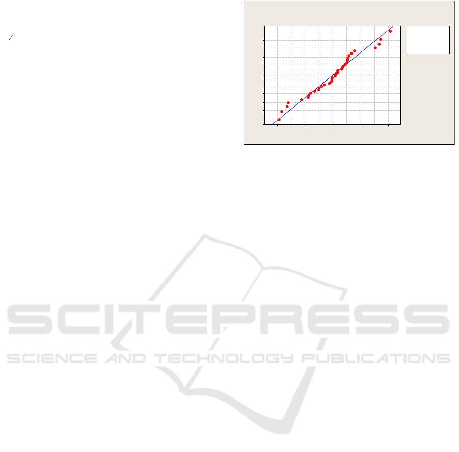
4.3.3 Normal Distributed Assumption Test

Normal distributed assumption test is performed by

the following Kolmogorov-Smirnov test.

: Data is normally distributed

: Data is not normally distributed

5.02.50.0-2.5-5.0

RESIDUAL

Percent

Mean - 1.67819E-14

StDev 2.346

N38

KS 0.109

P-Valu e >0.150

Probability Plot of Residual

Nor ma l

Figure 1. Probability plot normal residual.

Based on Figure 1, it is found that the red dots

spread close to the linear (normal) line meaning that

the data has been normally distributed. In addition, it

can also be seen from the value of P-Value is greater

0,15. So the decision that can be taken is Failed

Reject H

at a significant level (α) in the amount of

5%, that is, the data has fulfilled normal distributed

assumptions. Based on the results of the assumption

test, it can be concluded that the residuals in the

linear regression model (global) data have normal

distribution, but the identical and independent

assumptions are not met. So that spatial regression is

done with GWR approach.

4.4 Modeling of Spatial Regression of

Percentage of Poor People

Analysis using GWR method aims to determine the

variables that affect the percentage of poor people in

each location of observation that is the district / city

in the province of East Java. The first step to get the

GWR model is to determine the point of latitude and

longitude coordinates at each location, calculate the

euclidean distance and determine the optimum

bandwidth value based on Cross Validation (CV)

criteria. The next step is to determine the weighting

matrix with kernel function: Fixed Gaussian, Fixed

Bi-Square, Adaptive Gaussian, Adaptive Bi-Square

and estimates GWR model parameters. The

weighted matrix obtained for each location is then

used to form the model, so that different models are

obtained at each observation location.

The hypothesis test of the GWR model consists

of two tests, namely the GWR model conformity test

and the parameter significance test of the GWR

model. Here are the results of hypothesis testing

GWR model.

Geographically Weighted Regression for Prediction of Underdeveloped Regions in East Java Province Based on Poverty Indicators

903

kiik

=),( ;

(There was no significant difference

between the linear regression model

(global) and the GWR model)

1 :

At least, there is one

kiik

≠),( k = 1,

2, ….,9

(There is a significant difference between

the linear regression model (global) and the

GWR model)

Table 6. Estimated GWR on kernel function weight.

Stat

istic

Function weight

Fixed

Gaussia

Fixed

Bi-

square

Adaptive

Gaussian

Adaptive

Bi-

square*

5.560 5.049 5.989 1.995

0.829 0.852 0.797 0.998

AIC

185.676 184.839 186.017 -14185

Table 6 shows the comparison of estimated

GWR models with different weights. The GWR

model conformity test is performed by using the

difference of sum of residual squares of GWR model

and global regression model. The GWR model will

be significantly different from the global regression

model if it can significantly reduce the number of

residual squares. Table 6 shows that the smallest

AICc value is the GWR model with the Adaptive Bi-

Square kernel function weights, that is -14185. So,

by using the level of significance α at 5% it can be

concluded that the GWR model is significantly

different from the global regression model. This

means that the GWR model with the Adaptive Bi-

Square kernel function weights more feasible to

describe the percentage of poor people in East Java

Province.

Next is a test of the significance of GWR model

parameters with Adaptive Bi-Square kernel function

weights partially to know which parameters

significantly influence the percentage of poor people

in each location of observation. The grouping of

districts with the same variables that significantly

affect the percentage of poor people is presented in

Table 7.

Table 7. T-count value in variables in each regency / city

using adaptive bisquare.

Regency/City

Predictor Variable

X1 X2 X3 X4

"Pacitan

Regency"

-0.58 0.69 -0.53 -2.89*

"Ponorogo

Regency"

0.46 -0.39 0.51 -3.06*

"Trenggalek

Regency"

1.22 -0.33 -0.24 -1.69

"Tulungagung

Regency"

2.31* 0.35 -0.88 -2.48*

"Blitar

Regency"

-1.73 0.92 -2.99* -0.39

"Kediri

Regency"

1.22 -0.07 -0.83 -0.67

"Malang

Regency"

1.37 -1.03 -1.41 -0.48

"Lumajang

Regency"

2.73* 1.22 -1.53 -2.76*

"Jember

Regency"

0.97 0.11 -1.36 -0.60

"Banyuwangi

Regency"

-0.44 0.78 -0.74 -2.85*

"Bondowoso

Regency"

1.87 -1.50 1.55 -2.46*

"Situbondo

Regency"

2.92* -0.74 1.50 -1.64

"Pasuruan

Regency"

-0.01 -0.51 0.32 -1.80

"Probolinggo

Regency"

-0.05 0.95 -1.10 -2.97*

"Sidoarjo

Regency"

3.02* -0.92 1.61 -2.00*

"Mojokerto

Regency"

0.46 0.10 -0.14 -1.00

"Jombang

Regency"

1.36 0.82 -1.17 -0.89

"Nganjuk

Regency"

0.55 -0.08 1.05 -1.16

"Madiun

Regency"

2.92* 0.67 -1.13 -2.97*

"Magetan

Regency"

1.06 -1.16 0.10 -0.61

"Ngawi

Regency"

0.50 -3.55* 0.60 1.72

"Bojonegoro

Regency"

-2.41* 2.43* -2.84* 0.38

ICPS 2018 - 2nd International Conference Postgraduate School

904

5 CONCLUSIONS

Result of modeling percentage of poor population in

East Java Province based on Regency / City using

linear regression showed that only one variable that

affect the percentage of poor people, which is

literacy rate. The percentage of poor people in East

Java Province spread spatially because there is

heterogeneity between observation locations which

means that the observation of a location depends on

the observation in other location with adjacent

distance so spatial regression modeling with

Adaptive Bisquare kernel function was done, which

produced 9 groups.

REFERENCES

Anselin, L., 1988. Spatial Econometrics: Method and

Models. Netherlands, Kluwer Academic Publishers.

Chasco, C., Garcia, I., and Vicens, J., 2007. Modeling

Spatial Variations in Household Disposible Income

with Geographically Weighted Regression. Munich

Personal RePEc Arkhive (MPRA) Working Papper

No. 1682.

Draper, N., Smith, H., 1992. Analisis Regresi Terapan.

Jakarta, PT Gramedia Pustaka Utama

Fotheringham, A.S., Brunsdon, C., and Charlton, M.,

2002. Geographically Weighted Regression. Jhon

Wiley & Sons, Chichester, UK

LeSage, J.P., 2001. A Family of Geographically Weighted

Regression. Departement of Economics University of

Toledo.

Leung, Y., Mei, C.L., and Zhang, W.X., 2000a. Statistic

Tests for Spatial Non-Stationarity Based on the

Geographically Weighted Regression Model,

Environment and Planning A, 32 9-32.

Leung, Y., Mei, C.L., and Zhang, W.X., 2000b. Testing

for Spatial Autocorrelation Among the Residuals of

the Geographically Weighted Regression.

Environment and Planning A, 32, 871-890.

Miller, H.J., 2004. Tobler’s First Law and Spatial

Analysis. Annals of the Association of America

Geographers, 94(2), 284-289.

APPENDIX

Group 1: Regency / City di in East Java with

Percentage of Poor People Not Affected by Literacy

Rate

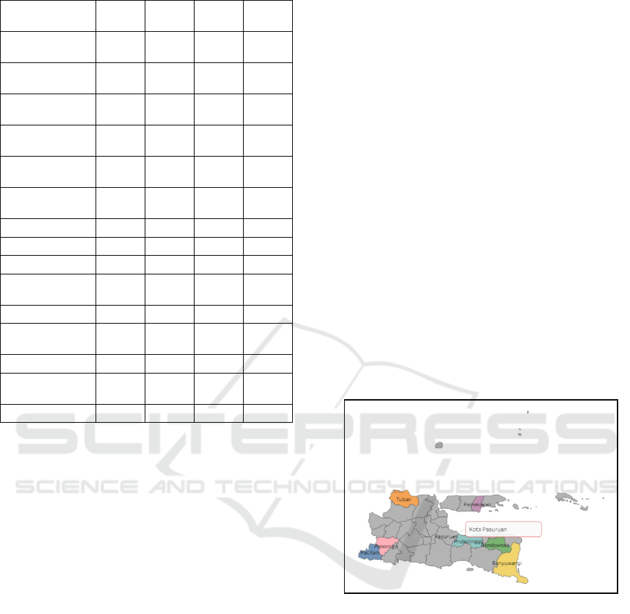
Group 2: Regency / City in East Java with

Percentage of Poor People Not Affected by Life

Expectancy Factors, Average School Duration, Per

Capita Population Expenditure, and Literacy Rate

"Tuban

Regency"

1.81 0.35 -0.93 -2.19*

"Lamongan

Regency"

-1.80 0.01 0.47 1.48

"Gresik

Regency"

3.14* -5.10* 2.16* 1.99*

"Bangkalan

Regency"

-2.10* 0.28 -0.22 -2.63*

"Sampang

Regency"

3.37* -3.91* 3.84* 2.83*

"Pamekasan

Regency"

0.01 0.83 -0.90 -3.00*

"Sumenep

Regency"

2.90* 1.59 0.13 -2.68*

"Kediri City" 1.54 0.19 -1.43 -0.95

"Blitar City" -1.15 1.24 -1.36 -1.69

"Malang City" 0.32 0.96 -1.28 -1.56

"Probolinggo

City"

2.90* 1.59 0.09 -2.68*

"Pasuruan City" -0.15 0.92 -1.08 -3.05*

"Mojokerto

City"

0.82 -0.09 1.08 -1.13

"Madiun City" 2.20* -1.33 0.72 -2.00*

"Surabaya

City"

-0.69 -4.77* 3.48* 3.41*

"Batu City" 3.22* -5.15* 2.23* 2.04*

Geographically Weighted Regression for Prediction of Underdeveloped Regions in East Java Province Based on Poverty Indicators

905

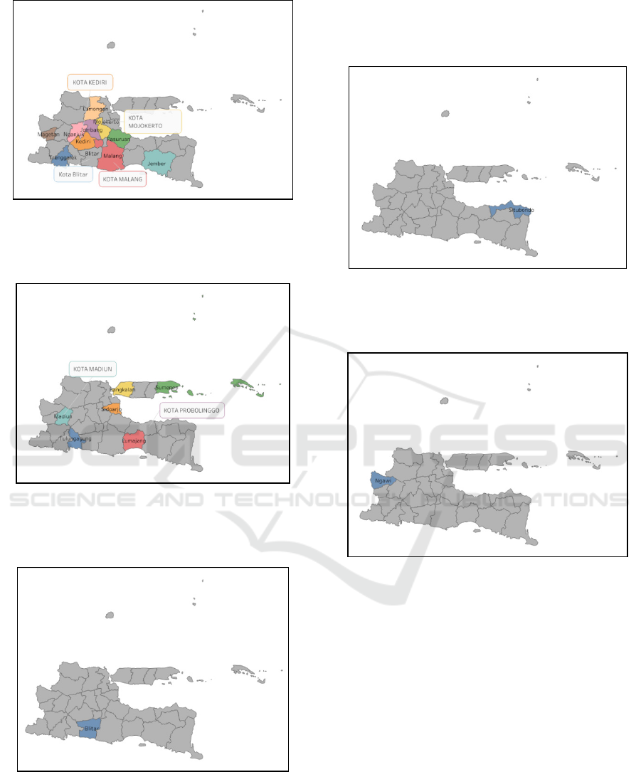
Group 3: Regency / City in East Java with

Percentage of Poor People Affected by Life

Expectancy Figures and Literacy Rates

Group 4: Regency / City in East Java with

Percentage of Poor People Affected by Capita

Population Expenditure

Group 5: Regency / City in East Java with

Percentage of Poor People Affected by Life

Expectancy Factor

Group 6: Regency / City in East Java with

Percentage of Poor People Affected by Average

School Duration

Group 7: Regency / City in East Java with

Percentage of Poor People Affected by Average

School Duration, Per Capita Population Expenditure,

and Literacy Rate

ICPS 2018 - 2nd International Conference Postgraduate School

906

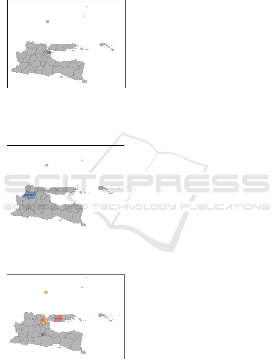
Group 8: Regency / City in East Java with

Percentage of Poor People Affected by Life

Expectancy Factors, Average School Duration, Per

Capita Population Expenditure, and Literacy Rate

Group 9: Regency / City in East Java with

Percentage of Poor People Affected by Life

Expectancy Factors, Average School Duration, and

Per Capita Population Expenditure

Geographically Weighted Regression for Prediction of Underdeveloped Regions in East Java Province Based on Poverty Indicators

907