
New Depth-averaged Non-hydrostatic Hydrodynamic Model
for Flows over a Slope
Z Jing
1
, H Q Cao
2, *
, H P Luo
3
, W L Zhai
4
and K F Zhao
5
Basin Water Environmental Research Dept., Changjiang River Scientific, Research
Institute, Wuhan 430010, China
Corresponding author and e-mail: H Q Cao, 673844316@qq.com
Abstract. Compared to the hydrostatic hydrodynamic model, the non-hydrostatic
hydrodynamic model can accurately simulate flows which have obvious vertical accelerations.
This paper proposes a non-hydrostatic hydrodynamic model. The horizontal momentum
equation is obtained by integrating the Navier-Stokes equations from the bottom to the free
surface. The vertical momentum equation is approximated by the Keller-box scheme. A non-
hydrostatic correction method is used to solve the model equations. The proposed model is
verified using measurements from a solitary wave experiment, and good consistency is
reported. The results show that the proposed model is an effective tool for simulation of
coastal engineering.
1. Introduction
The propagation of sea waves over a slope involves a series of complex physical processes such as
wave refraction, wave diffraction, and shoaling. Many mathematical models were used to analyze the
prototype experiments of wave propagation and transformation, including the Boussinesq-type
equation [1], potential flow model, and non-hydrostatic hydrodynamic model.
Compared to hydrostatic models, non-hydrostatic models consider the effect of dynamic pressure,
and are thus appropriate for situations with significant vertical acceleration. Thus non-hydrostatic
models are particularly well-suited to grasping the discipline of complex flow movement. Managing
the dynamic pressure variable is the key to successful non-hydrostatic modeling. In most non-
hydrostatic models, it is assumed that the pressure of the surface grid conforms to the hydrostatic
distribution and the dynamic pressure variables are placed at the center of the surface grid [2, 3].
Thus these models don’t completely deviate from the hydrostatic assumption.
To solve the problem, this paper proposes a novel non-hydrostatic hydrodynamic model. Based on
a non-hydrostatic correction method, the horizontal momentum equation is obtained by integrating
the Navier-Stokes equations from the bottom to the free surface. The vertical momentum equation is
approximated by Keller-box scheme. The validity of the model was verified by a solitary wave
experiment.
2. Mathematical model
To improve the hydrostatic hydrodynamic model, the pressure term in the 3D Navier-Stokes (N-S)
equations is separated into hydrostatic and non-hydrostatic components. The horizental momentum
Jing, Z., Cao, H., Luo, H., Zhai, W. and Zhao, K.
New Depth-averaged Non-hydrostatic Hydrodynamic Model for Flows over a Slope.
In Proceedings of the International Workshop on Environmental Management, Science and Engineering (IWEMSE 2018), pages 133-139
ISBN: 978-989-758-344-5
Copyright © 2018 by SCITEPRESS – Science and Technology Publications, Lda. All rights reserved
133
equations and the continuity equation are integrated from bottom to free surface. The vertical
momentum equation only retains the dynamic pressure gradient term. Coupling with the kinematic
boundary conditions at the water bottom and free surface, a plane 2D, depth-integrated non-
hydrostatic hydrodynamic model is obtained [4].
0
U V w
x y z
(1)
( ) ( )
0
UH VH
t x y
(2)
2
2 2 2
4/3
cos
1
s a s
h
Cw
U U U q
U V g dz
t x y x H x H
n gU U V
H
(3)
2
2 2 2
4/3
sin
1
s a s
h
Cw
V V V q
U V g dz
t x y y H y H
n gV U V
H
(4)
1wq
tz
(5)
Where Eq. (1) is the continuity equation; Eq. (2) is the free surface equation; Eqs. (3)-(4) are the
horizental momentum equations (the Coriolis term is ignored); Eq. (5) is the vertical momentum
equation (the convective term and viscosity term are ignored). t is time (s); U and V (m/s) are the
depth-averaged velocity in the x and y directions, respectively; w is the velocity in the z direction
(m/s); ρ is water density (kg/m
3
); q is the dynamic (non-hydrostatic) pressure; H is the total water
depth (m), H=h+η; h is the still water depth (m); η is the surface elevation above the still-water level
(m); C
s
is the wind drag coefficient; ρ
α
is air density (kg/m
3
); w
s
is the wind speed (m/s); α is the
angle between the wind direction and the x direction; n is the roughness coefficient.
In the solitary wave propagation experiments, the flow field of the experiments presents lateral
uniformity of velocity; that is to say, the flow has significant velocity components only in the
longitudinal direction and the changes in the lateral direction are effectually negligible. Thus, a
longitudinal, 1D model is sufficient to simulate the flow motion accurately. Moreover, as opposed to
the strong disturbance caused by the wave generator at the entrance, the water surface and the friction
force at the bottom of the tank can be ignored as the indoor air velocity and the friction force of the
bottom plate of the water tank are low in these prototype experiments. From the above, the variations
in velocity in the lateral direction, the wind shear force and the bottom friction force can be ignored,
and the 2D non-hydrostatic model equations can be simplified as follows:
0
Uw
xz
(6)
()
0
UH
tx
(7)
1
h
U U q
U g dz
t x x H x
(8)
The integration of the dynamic pressure gradient adopts an approximate expression:
1 1 ( )
22
b
b
h
q
qh
dz H q
x x x
(9)
IWEMSE 2018 - International Workshop on Environmental Management, Science and Engineering
134
Where q
b
is the dynamic pressure at the bottom, substituting Eq. (9) into Eq. (8), we obtain:
1 ( )
22
bb
qq
U U h
Ug
t x x x H x
(10)
Eqs. (6), (7), (10) and the vertical momentum equation Eq. (5) compose the governing equations
of depth-integrated 1D non-hydrostatic hydrodynamic model.
3. Numerical solution
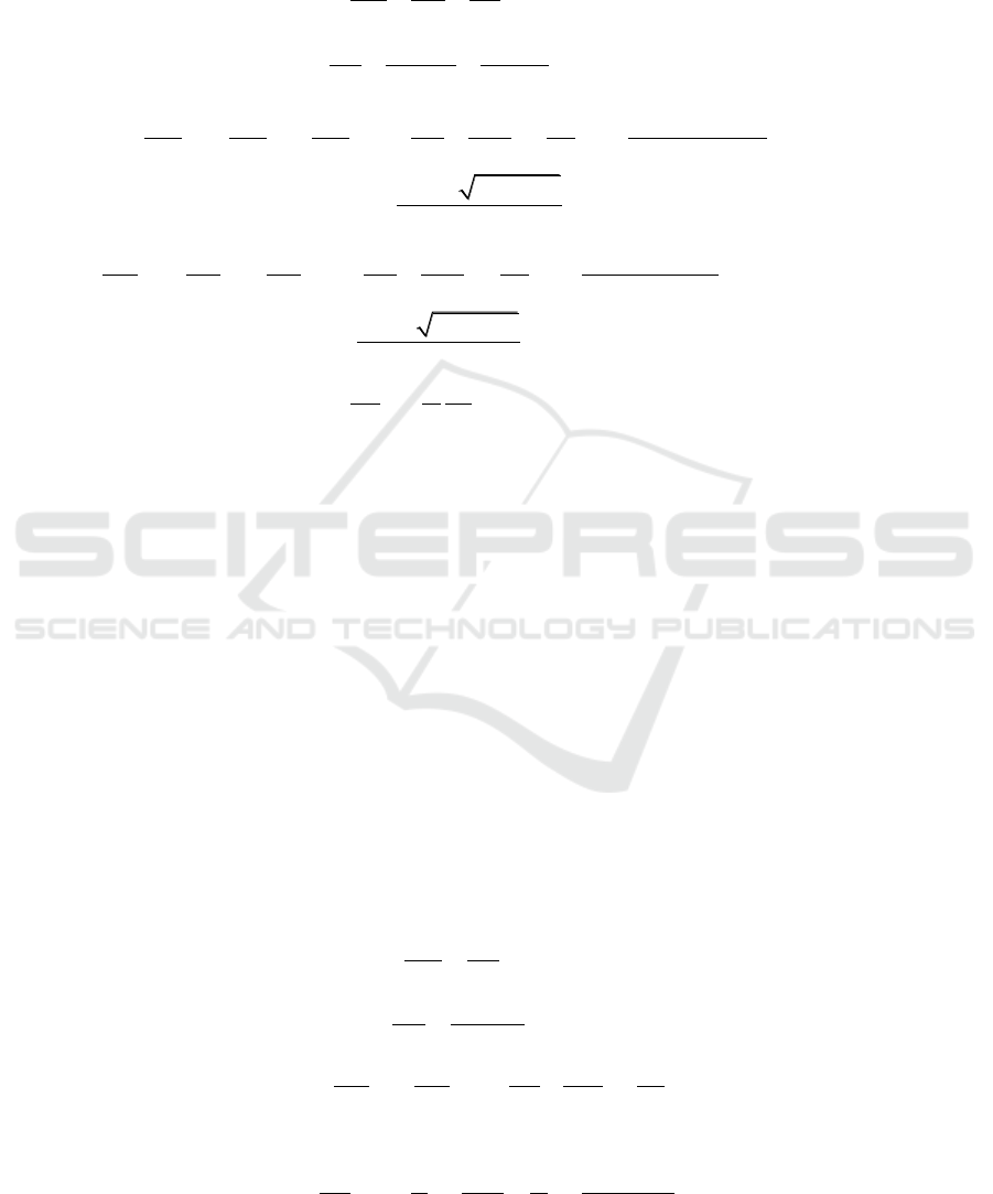
A structured C-grid scheme is used for discretization of the computational domain. The governing
equations are solved by the finite difference method (FDM). Figure 1 shows the layout of variables. i
denotes the cell grid centre in the x direction; U is defined at the centre of the grid faces (i ± 1/2); η, h,
and H are located at the centre of the grid; The dynamic pressure q is located at the centre of the top
and bottom surfaces; the dynamic pressure at the bottom q
b
is at the centre of the bottom surface; the
dynamic pressure at the free surface is set to be zero in order to satisfy the zero dynamic pressure
condition; W
S
and W
B
, which are the vertical velocity at the free surface and bottom, are located at the
centre of the top and bottom surfaces, respectively.
x
x
U
i-1/2
U
i-1/2
W
S_i
W
S_i
η
i
, h
i
, H
i
η
i
, h
i
, H
i
z
z
U
i+1/2
U
i+1/2
W
B_i
W
B_i
q
b_i
q
b_i
Figure 1. Layout of variables.
All the terms except the dynamic pressure gradient term in Eq. (10) are solved explicitly by
central difference scheme. The dynamic pressure gradient term is solved by implicit scheme. Where
superscript n and (n+1) denote the time levels n and (n+1), respectively; Δt and Δx denote the time
step and the space step, respectively. The discrete form Eq. (10) can be written as:
1
1/2 1/2 1/2 3/2 1/2 1
_ 1 _ 1 1
11
_ 1 _
1
( ) ( )
2
( )( )
( )
2
n n n n n n n
i i i i i i i
n n n n
b i b i i i i i
nn
b i b i
nn
ii
tt
U U U U U g
xx
q q h h
tt
qq
x H H x
(11)
A non-hydrostatic correction method is used for solving Eq. (11):
The hydrostatic step
In the first step, Eq. (12) retain the convective term, the water level gradient term, the combination
term of dynamic pressure and water level can be obtained. The intermediate value of the velocity
(denoted as U
n+1/2
) can be calculated by solving Eq. (12).
New Depth-averaged Non-hydrostatic Hydrodynamic Model for Flows over a Slope
135

1
1/2 1/2 1/2 3/2 1/2 1
_ 1 _ 1 1
1
( ) ( )
2
( )( )
2
n n n n n n n
i i i i i i i
n n n n
b i b i i i i i
nn
ii
tt
U U U U U g
xx
q q h h
t
x H H
(12)
The non-hydrostatic step
Based on the calculated U
n+1/2
in the hydrostatic step, Eq. (12) only retain the dynamic pressure
gredient term and Eq. (13) can be obtained:
1 1/2 1 1
1/2, 1/2, _ 1, _ ,
()
n n n n
i j i j b i j b i j
t
U U q q
x
(13)
The Keller-box scheme is used to discretize the vertical momentum equation Eq. (5) [5]. This
scheme has three steps. First, by the forward differencing scheme at the centre of the bottom face, the
dynamic pressure gradient term can be approximated as:
(14)
Second, the dynamic pressure gradient term is discretized at the centre of the upper face by the
backward diff erencing scheme as follows:
(15)
Finally, we take the average of Eqs. (14) and (15) as the final discrete form of Eq. (5) as follows:
(16)
Where W
B
n+1
is evaluated in terms of the kinematic boundary condition at the bottom [6]:
(17)
The continuity equation Eq. (6) is discretized as:
(18)
Substituting Eqs. (13), (16) and (17) into Eq. (18) gives Eq. (19):
(19)
The coefficients of Eq. (19) could be known. They form a system of a linear tri-diagonal matrix
equation, namely the Pressure Poisson Equations (PPEs). q
b
n+1
could be calculated by solving the
PPEs using TMDA method. Substituting q
b
n+1
into Eqs. (13) and (16) gives U
n+1
and W
S
n+1
. The free
surface η can be updated from the discrete form of Eq. (20):
1 1 1
_ _ _ _
0
11
n n n n
B i B i b i b i
nn
ii
W W q q
t H H
1 1 1
_ _ _ _
,
0
11
n n n n
S i S i b i b i
nn
i j i
W W q q
t H H
1 1 +1
_ _ _ _ _
2
+
n n n n n
S i b i S i B i B i
n
i
t
W q W W W
H
1 1/2 1/2 1/2 1/2
_ 1 1/2 1/2 1/2 1/2
1/2 1/2 1/2 1/2
1 1/2 1/2 1/2 1/2
1
( )( )
4
1
( )( )
4
n n n n n
B i i i i i i i
n n n n
i i i i i i
W h h U U U U
x
h h U U U U
x
- - + + +
- - + - +
11
11
__
1/2 1/2
0
nn
nn
S i B i
ii
n
i
WW
UU
xH
1 1 1
_ 1 _ _ 1
n n n
T b i T b i T b i T
B q C q T q F
IWEMSE 2018 - International Workshop on Environmental Management, Science and Engineering
136
1 1 1
1/2 1 1/2 1
[ ( )- ( )]
2
n n n n n n n n
i i i i i i i i
t
U H H U H H
x
(20)
4. Model verification
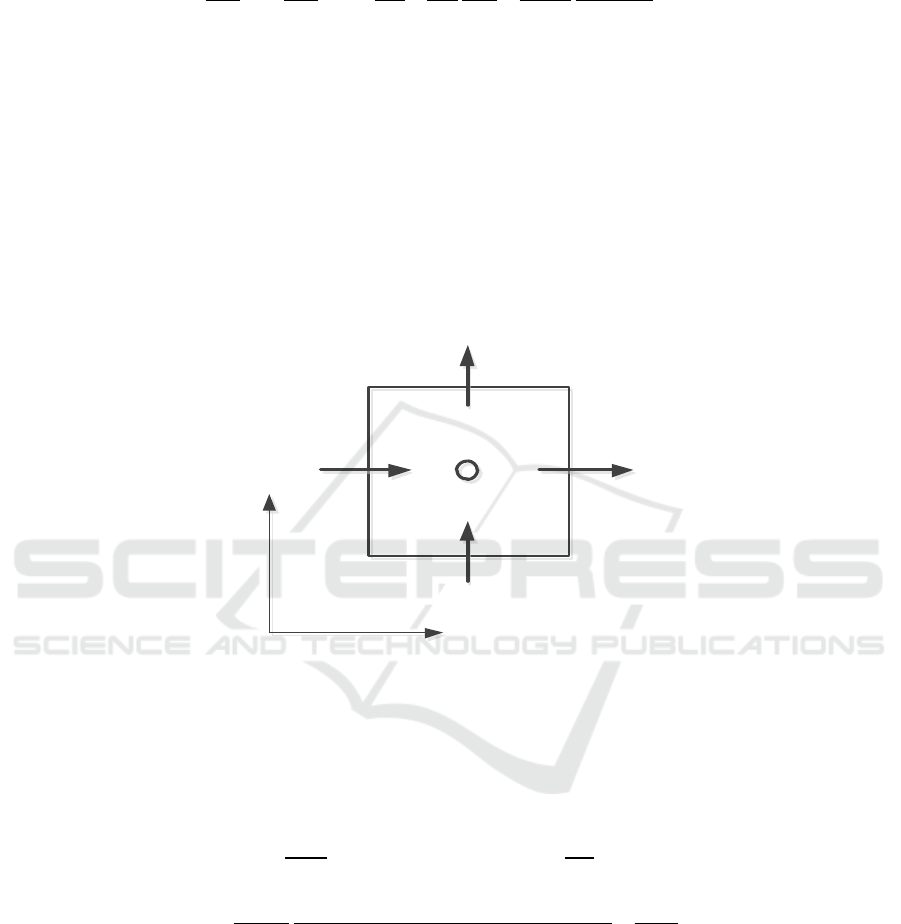
The process of wave propagation on an underwater submerged breakwater is very complex. It is
commonly used to verify non-hydrostatic models. The proposed model was verified for solitary wave
experiment by Madsen.
Madsen and Mei made an experimental setup to study the solitary wave shoaling over a
submerged bar, as shown in Figure 2 [7]. There was a slope which was 200cm far from the left side
of the channel. The solitary wave propagates from a constant depth h
1
=7.62 cm to a smaller constant
depth h
2
=3.81 cm through a slope. There were four stations, A, B, C, and D (x=159.36cm, 276.2 cm,
365.1cm, 423.52cm), observing the free surface. The initial position of the wave crest was at x=-
80cm, and its amplitude was 0.9144cm. The size of the simulation region is 600cm and the
simulation time is 10s; Δx=5cm; Δt=0.001s.
Figure 2. Sketch of the experiment set-up of Madsen.
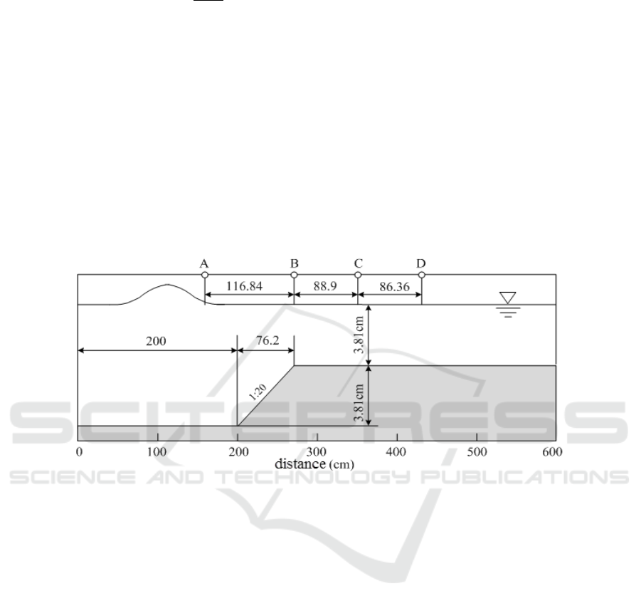
Figure 3 presents the measured values and the simulated values of the non-hydrostatic and
hydrostatic models at four monitoring stations: Station A, B, C, and D. Oscillation occurs in the
hydrostatic simulated results at Stations B, C, and D. The main reason for dispersion is that solitary
wave splits into a series of short waves when it is under dynamic pressure. After the short waves pass
through these three monitoring stations, decreased dynamic pressure, declined dispersion, and
disappeared oscillation occur. Clearly, then, the hydrostatic model cannot correctly reflect the short
wave and its dispersion effect as the influence of the dynamic pressure is ignored. The simulated
results of the non-hydrostatic model closely coincide with the measured data. In short, it effectively
simulates the process of solitary wave propagation over a slope.
New Depth-averaged Non-hydrostatic Hydrodynamic Model for Flows over a Slope
137
Figure 3. Simulated η/h
1
by the non-hydrostatic (solid line) and hydrostatic model (dotted line);
experimental data (circled) in Stations A, B, C and D.
5. Conclusions
This paper proposes a novel non-hydrostatic hydrodynamic model based on a non-hydrostatic
correction method. With the pressure divided into hydrostatic and dynamic components, the
horizontal momentum equation is obtained by integrating the Navier-Stokes equations from the
bottom to the free surface. The vertical momentum equation is approximated by the Keller-box
scheme. All the terms except the dynamic pressure gradient term in the horizontal momentum
equation are solved explicitly by central difference scheme. The dynamic pressure gradient term is
solved by implicit scheme. The validity of the model was verified by a solitary wave propagation
experiment over a slope, and good consistency is reported. The model is suitable for application to
lab experiment. However, the depth-averaged model should be expanded to 3D model if more
detailed 3D flow field is required.
Acknowledgement
This work was supported by Hubei Provincial Natural Science Foundation of China (2016CFA092)
and Major Science and Technology Program for Water Pollution Control and Treatment of China
(2017ZX07108-001).
References
[1] Beji S and Battjes J A 1994 Numerical simulation of nonlinear wave propagation over a bar
Coastal Engineering vol 23 pp 1-16
[2] Casulli V and Stelling G 1998 Numerical simulation of 3D quasi-hydrostatic, free-surface
flows Journal of Hydraulic Engineering vol 124(7) pp 678-686.
[3] Zhou J G and Stansby P K 1998 An arbitrary Lagrangian-Eulerian σ (ALES) model with non-
hydrostatic pressure for shallow water flow Computational Methods in Applied Mechanics
and Engineering vol 178(1-2) pp 199-214
[4] Guo X M, Kang L and Jiang T B 2013 A new depth-integrated non-hydrostatic model for free
surface flows SCIENCE CHINA Technological Sciences vol 56(4) pp 824-830
[5] Keller H B 1971 A new difference scheme for parabolic problems Numerical Solutions of
Partial Differential Equations II Hubbard B (ed.) Academic Press: New York pp 327-350
t (s) t (s)
t (s) t (s)
IWEMSE 2018 - International Workshop on Environmental Management, Science and Engineering
138

[6] Yamazaki Y, Kowalik Z and Cheung K F 2009 Depth-integrated, non-hydrostatic model for
wave breaking and run-up International Journal for Numerical Methods in Fluids vol 61(5)
pp 473-497
[7] Madsen O S and Mei C C 1969 The transformation of a solitary wave over uneven bottom.
Journal of Fluid Mechanics vol 39(4) pp 781-791
New Depth-averaged Non-hydrostatic Hydrodynamic Model for Flows over a Slope
139
