Classification of Soil Types Using Hyperspectral Imaging
Technology
S Y Jia
1,
H Y Li
1, 2
, C X Miao
1
and Q Li
1,*
1
College of Mechanical and Electrical Engineering, China Jiliang University,
Hangzhou, PR China
2
College of Computer Science and Technology, Zhejiang University of Technology,
Hangzhou, PR China
Abstract. Soil type is a key indicator in field survey, but the current soil classification
method largely depends on personal experiences of operators. In this work, hyperspectral
imaging (HSI) technology was applied for the fast and accurate classification of soil types. A
total of 183 soil sa mples collected from Shangyu City, People’s Republic of Ch ina, were
scanned by a near-infrared hyperspectral imaging system with the wavelength range of 874-
1734 nm. The soil samples belonged to three major soil types of this area, included paddy soil,
red soil and seashore saline soil. The method of successive projections algorithm (SPA) was
utilized to select effective wavelengths from the full spectrum. Pattern texture features
(energy, contrast, homogeneity and entropy) were extracted from the gray-scale images at the
effective wavelengths. The method of support vector machines (SVM) was used to establish
classification models. The results showed that: using the combined data sets of effective
wavelengths and texture features for modelling reached the optimal correct classification rate
of 91.8%. The results indicated that hyperspectral imaging technology could be used for soil
type classification, and data fusion combining spectral and image texture information showed
advantages for the classification of soil types.
1. Introduction
Soil classification is important for soil management and sustainable land utilization [1]. Different
soils have different compositions and different environmental and physical properties [2]. At present,
Munsell card is the most commonly used soil classification method, which applied soil color to
distinguish soil categories. However, this card divides the color space into different small sections, it
is not convenient to acquire large amounts of data with modern digital technologies [3]. Meanwhile,
this method largely depends on personal experiences, which are easily to cause errors.
Developed from remote sensing, hyperspectral imaging (HSI) has gained extensive attentions
from different fields such as food [4], agriculture [5] and medical science [6]. Through each
measurement by the HSI instrument, both the spectral information and image texture information of
the sample can be obtained. Spectra can reflect the molecular structure and composition of the tested
samples. Image texture, which is characterized by the relationship of the intensities of neighboring
pixels, has been successfully used for the classification of fruit ripeness [7], fish freshness [8] and
502
Jia, S., Li, H., Miao, C. and Li, Q.
Classification of Soil Types Using Hyperspectral Imaging Technology.
In Proceedings of the International Workshop on Environmental Management, Science and Engineering (IWEMSE 2018), pages 502-511
ISBN: 978-989-758-344-5
Copyright © 2018 by SCITEPRESS – Science and Technology Publications, Lda. All rights reserved

plant disease degree [9]. Cai, et al. used image texture features to classify soil samples with different
degrees of salinization, and a higher correct classification rate has been obtained [10]. They
considered that when the soil samples were similar in spectral features, texture features would play a
positive role in the sample recognition, and combined the information of spectral and texture features
can help to improve the classification accuracy. Ma, et al. using HSI technique to distinguish healthy,
greening disease infected and zinc-deficient citrus [9]. As the leaf spectra of greening disease
infected and zinc-deficient citrus were partially overlapped, and the leaf texture features of greening
disease infected and zinc-deficient citrus were similar, utilization of spectral information or texture
features for modelling cannot achieve good classification results. However, data fusion combining
spectral information and texture features greatly improved the correct classification rate for the three
kinds of citrus. To our knowledge, comprehensive utilization of spectral information and image
texture features for the classification of soil types was seldom reported.
Hyperspectral image generates an immense amount of data. Some of them may contribute more
co-linearity, redundancies, and noise than relevant information to calibration models, which is a huge
challenge for the application of HSI technique [11]. Effective wavelength selection, aiming to select
only a few wavelengths which carry the most of useful information with minimum collinearity and
redundancy from full spectrum, is believed to reduce amount of data, computational task, and build a
simple and robust model [12, 13]. Successive projections algorithm (SPA) is a popular tool for
wavelength selection in multivariate calibration and classification [14]. It is able to select a small
representative set of spectral wavelengths with a minimum of collinearity. In machine visual systems,
the most popular method for texture feature analysis is Gray level co-occurrence matrix (GLCM)
method [15]. GLCM, created through calculating how often a pixel with a particular gray level value
occurs at a specified distance and angle from its adjacent pixels, is able to take into account the
specific position of a pixel relative to another. In this work, SPA and GLCM were adopted to select
effective wavelengths and extract texture features, respectively.
The objective of this work was to investigate the feasibility of classifying soil types using HSI
technique. The specific objective was to build classification models for soil types in utilization of
spectral information and image texture features.
2. Materials and methods
2.1. Soil samples and laboratory reference measurement
Total 183 soil samples sampled from the upper soil layer (0-30 cm) of Shangyu City, Zhejiang
province, People’s Republic of China, were used in this study. All the samples were air dried and
sieved with a diameter of 1 mm. Then they were air dried again at 60°C for 48 h. A small portion of
each sample was sent to the agricultural testing center of Zhejiang Provincial Academy of
Agricultural Sciences (ZPAAS) for soil classification analyses. The remaining samples were used for
HSI measurement.
According to the classification and codes for Chinese soil (National standard of China,GB/T
17296–2009), the soil samples belonged to three major soil types of this area, namely, paddy soil (84
samples), red soil (57 samples) and seashore saline soil (42 samples).
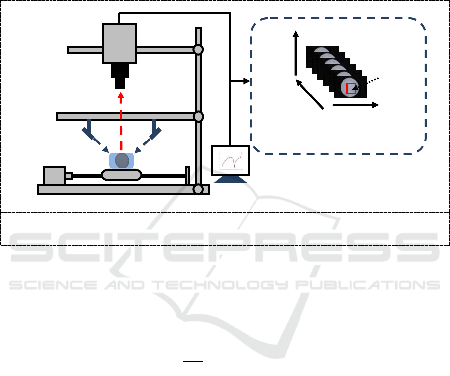
2.2. Hyperspectral image acquisition
The hyperspectral images of soil samples were captured by a near-infrared HSI system with the
wavelength range of 874-1734 nm and 256 bands. The system was composed of an imaging
spectrograph (ImSpector N17E; Spectral Imaging Ltd., Oulu, Finland), a CCD camera (Xeva 992;
Xenics Infrared Solutions, Leuven, Belgium), two 150W quartz tungsten halogen lamps (Fiber-Lite
DC950 Illuminator, Dolan Jenner Industries Inc., USA), and a conveyer belt which was driven by a
stepper motor for sample movement (Figure 1). The entire system was fixed in a darkroom. The soil
Classification of Soil Types Using Hyperspectral Imaging Technology
503

samples were put into petri dishes with a diameter of 60 mm. The petri dishes were placed on the
conveyer belt for image acquisition. Hyperspectral image provided both spectral and image
information simultaneously. Each pixel within the hyperspectral image contained a spectrum at the
spectral range of the system, and there was a gray-scale image at each wavelength.
Figure 1. Schematic diagram of the hyperspectral imaging system. This system can obtain images
in the spectral region of 874-1734 nm.
To acquire clear and non-deformable hyperspectral images, the moving speed of the conveyer belt,
the exposure time of the camera, and the height between the lens of the camera and the sample were
set as 24 mm/s, 3 ms, and 30.8 cm, respectively.
Raw hyperspectral image (I0) was corrected by white (W) and dark (D) reference images. The
white reference image was obtained using a standard Teflon tile (~99.9% reflectance), and the dark
reference image was acquired by turning off the light source and covering the camera lens with its
opaque cap. The corrected image (I) was calculated by the following equation:
 




  (1)
2.3. Spectral data extraction and effective wavelength selection
For each soil sample’s hyperspectral image, the region that covered the petri dish without the edge
was selected as the region of interest (ROI). The reflectance values of all pixels in the ROI were
averaged to generate only one mean spectrum. Then, the mean spectrum was reduced to 975-1645
nm to eliminate noise at edges, which was used to represent the spectral data of one sample. The
same procedure was repeated for all ROI images, and a full spectrum matrix 237 samples × 200
bands was constructed.
Effective wavelengths were selected by the SPA method. The best variable subset was determined
on the basis of the root mean square error of leave-one-out cross validation in the calibration set
(RMSECV). A detailed description of SPA can be found in literature [16,17].
2.4. Texture variable extraction
In creating the GLCM, the direction of 0°, 45°, 90° and 135°and distance of one pixel were applied,
and four popular texture variables, such as energy, contrast, homogeneity and entropy were
Came ra
Spectrograph
Lens
Light Source
Stepper
Motor
Conveyer
Belt
Sample
No. of pixels
in X direction
No. of
pixels
in Y
directio
n
Heperspectral Image
Computer
Region of
Interest
(ROI)
Wavelengths
IWEMSE 2018 - International Workshop on Environmental Management, Science and Engineering
504

calculated in each direction based on GLCM [18,19] . The mean values of the four directions were
used, and four averaged texture variables were obtained from the ROI of one gray-scale image. As
the hyperspectral image contained gray-scale images at continuous wavelength bands, a total of 200
gray-scale images have been obtained from a single measurement of one soil sample. Extracting
texture features from each gray-scale image would generate a large amount of redundant information
which was not useful for modelling. Hence, texture features were only extracted from the gray-scale
images at effective wavelengths.
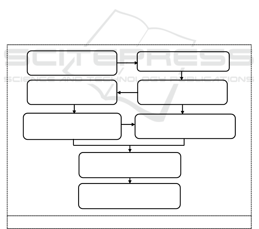
2.5. Establishment of classification and regression models
The main steps of the work were shown in fig ure 2. After hyperspectral image acquisition, correction
and reflectance extraction, the samples of each soil type were randomly spilt into the calibration set
and prediction set at a ratio of 2:1 so as to establish classification models: the calibration set was
composed of 56 paddy soil samples, 38 red soil samples and 28 seashore saline soil samples, while
the prediction set included the remaining 28 paddy soil samples, 19 red soil samples and 14 seashore
saline soil samples. Then the method of SPA was used to select effective wavelengths based on the
calibration set. The reference data y in SPA was category value. The samples of paddy soil, red soil
and seashore saline soil were assigned category values of 1, 2 and 3. After effective wavelength
selection, texture features were extracted by GLCM. The method of support vector machines (SVM)
was used to establish classification models based on the effective wavelengths and texture features.
SVM has been proved as a reliable method for classification, dealing with both linear and nonlinear
data efficiently [20, 21]. In this work, radial basis function kernel was selected as the kernel function,
which is the typical general-purpose kernel.
Figure 2. Main steps of this work.
Hyperspectral image correction
Hyperspectral image acquisition for
soil samples
Identification of region of interest
(ROI)
Reflectance extraction
Wavelength selection by successive
projections algorithm (SPA)
Texture features extracted by Gray level
co-occurrence matrix (GLCM)
Classification models established by
support vector machine (SVM)
Classification for soil types
Classification of Soil Types Using Hyperspectral Imaging Technology
505

2.6. Software
The hyperspectral image analysis was conducted on ENVI 4.6 (ITT, Visual Information Solutions,
Boulder, CO, USA) and Matlab 2010 (The Math Works, Natick, MA, USA). The methods of SVM,
SPA were operated in Matlab 2010 .
3. Results and discussion
3.1. Spectral profiles
Figure 3 showed the RGB images of three soil type samples. It can be noted that the surface of
seashore saline soil was rougher than that of paddy soil and red soil. As can be seen in figure 4 (a),
the average spectrum of each soil type in the range of 975-1645 nm showed similar trend. The
significant peaks around 1400 nm appeared in all spectra, which were attributed to the absorption of
water in soil. There were some differences in the average spectral baselines. The reflectance value of
seashore saline soil was lower than that of paddy soil and red soil, mainly because the light scattering
of the surface of seashore saline soil was too intense.
Figure 3. RGB images of paddy soil, red soil and seashore saline soil samples.
In order to examine the structure of the spectral data, a principal components analysis was
performed on the full spectrum matrix. The principal components analysis scores were submitted to
Fisher’s linear discriminant analysis (LDA). Because the first four principal components (PCs) of the
spectral data can explain nearly 100% of total variance, they were set as input of LDA. Figure 4 (b)
showed the samples of paddy soil, red soil and seashore saline soil distinguished by the score plot of
Fisher's LDA. The correct classification percentage was 85%. It can be observed that the samples of
paddy soil and seashore saline soil were relatively well grouped, while some red soil samples were
mixed with the samples of the other two soil types.
(b) Red soil
(a) Paddy soil
(c) Seashore saline soil
IWEMSE 2018 - International Workshop on Environmental Management, Science and Engineering
506

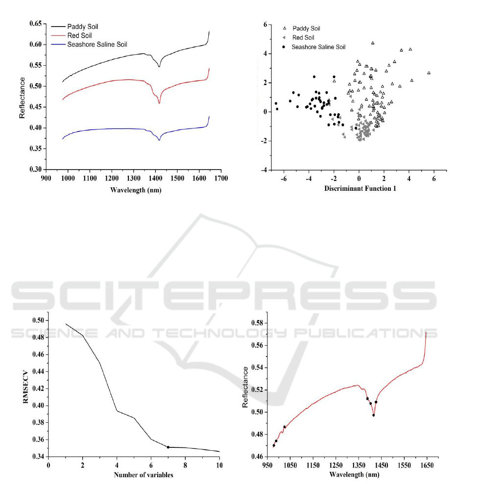
Figure 4. (a) The average spectrum of each soil type in the wavelength range of 975-1645 nm ; (b)
Grouping of 183 soil samples based on Fisher’s LDA using the first four principal components of
full spectrum matrix as input.
3.2. Effective variables selection
Figure 5. RMSECV curves with the number of variables selected by SPA for soil type
classification (a). The reference data in SPA was category value. The selected variables (shown as
dots) corresponding to raw spectra were presented in (b).
SPA was carried out to select effective variables from the full spectrum. The variation of RMSECV
with the number of selected variables for soil type classification is shown in figure 5 (a). Let
RMSECVmin be the minimum value in the RMSECV sequence. Seven variables were selected
through comparison of the RMSECV values which was not significantly larger than RMSEVmin by
(a)
(b)
(a)
(b)
Classification of Soil Types Using Hyperspectral Imaging Technology
507

applying the F-test criterion with a significance level α=0.25 [22]. Figure 5 (b) presented an overview
of the selected variables corresponding to raw spectra. The selected variables around the peak of
1400 nm can be approximately attributed to the absorption of water absorptions in the second
overtone region, while the variables selected in the wavelength range of 950-1050 nm were related to
overtones of aromatics C-H bond and amine N-H bond in organics [23]. This indicated that
considerable differences existed in moisture content and organic ingredients among the samples of
the three soil types.
3.3. Texture features extraction and analysis
ROI was defined as a rectangular area in the middle of the sample with 50*50 pixels (Figure 1). Four
texture features (Energy, contrast, homogeneity and entropy) based on GLCM at 7 effective
wavelengths were extracted, resulting in a total of 28 texture features (4 texture features × 7
wavelengths) obtained from the ROIs for each soil sample.
Figure 6 showed the mean values of the four texture features from different soil types. It can be
seen that energy and homogeneity of seashore saline soil was highest compared with the other two
soil types at the effective wavelengths, which indicated that the image texture of seashore saline soil
was rougher than that of the other two soil types [10]. The similar conclusion could be also obtained
by analyzing the mean values of contrast and entropy. They were the lowest for seashore saline soil,
which meant that the image texture of seashore saline soil contained less local variations. In general,
the texture features of seashore saline soil were clearly distinguished from those of the other two soil
types, and there were no intersections between the texture features of paddy soil and red soil,
although they were close at some effective wavelengths. Hence, it was possible for soil type
classification based on these statistics.
IWEMSE 2018 - International Workshop on Environmental Management, Science and Engineering
508

Figure 6. The mean texture features of different soil types at the effective wavelengths.
3.4. Classification for soil types
To build SVM models for soil type classification, the samples of paddy soil, red soil and seashore
saline soil were assigned category values of 1, 2 and 3. Table 1 showed the classification results of
SVM models using different input variables. When using spectral effective wavelengths for
modelling, it can be note that the discrimination accuracy was 88.5% for the calibration set and
83.6% for the prediction set. The results were similar with the classification performed on the full
spectrum matrix by LDA. Then, texture features were used for modelling. The discrimination
accuracy was 82.7% for the calibration set and 77.0% for the prediction set. The performances were
poorer compared with the model established by effective wavelengths. However, the samples of
seashore saline soil were well classified from the samples of the other two soil type.
Finally, both effective wavelengths and texture features were set as input for building SVM
models. As can be seen, the discrimination accuracy of the calibration set and prediction set were
both improved compared with the models using spectral effective wavelengths or texture features as
input. The samples of paddy soil and seashore saline soil were successfully classified, while some
samples of paddy soil and red soil were misclassified, and a few seashore saline soil samples were
(c)
(d)
(a)
(b)
Classification of Soil Types Using Hyperspectral Imaging Technology
509

misclassified as red soil samples. The results indicated that data fusion of combining effective
wavelengths and texture features showed advantages for the classification of soil types.
4. Conclusions
In this work, a HSI system covering the spectral range of 874-1734 nm was used to classify soil types.
The method of SPA was applied to select effective wavelengths from the full spectrum, and texture
features of energy, contrast, homogeneity and entropy were extracted from the gray-scale images at
the effective wavelengths. The classification models for soil types were established by the method of
SVM. The results showed that:
i. The classification model established by the combining data of effective wavelengths and texture
features achieved the optimal results for the classification of red, paddy and seashore saline soil
compared with the models established by the effective wavelengths or texture features. The correct
classification rate was 91.8 %.
ii. The overall results indicated that it was helpful to use image texture features for soil type
classification, and HSI technique could be used for soil type classification.
In future work, more soil samples with a wide range of soil types should be studied to build more
robust soil type classification models.
Acknowledgments
This work was supported by the Natural Science Foundation of Zhejiang Province, China (project no
LQ16F010006), the scientific research project of the education department of Zhejiang Province
(project no Y201533855 and Y201737559), and the key research and development plan of Zhejiang
Province (project no 2018C03040). The authors declare no conflict of interest.
Reference
[1] Hartemink A E and J Bockheim G 2013 Catena 104 251-256
[2] Viscarra Rossel R A, Minasny B, Roudier P and McBratney A B 2006 Geoderma 133 320-337
[3] Meyer R R and Kirkland A 1998 Ultramicroscopy 75 23-33
[4] Zhang C, Guo C, Liu F, Kong W, He Y and Lou B 2016 J. Food Eng. 179 11-18
Table 1. Classification results for soil types using SVM models established based on different
input variables.
Input variables
(c,g)
a
Calibration set
Prediction set
1
2
3
Accuracy
1
2
3
Accuracy
Effective
wavelengths
(23.12, 2.42)
1
51
4
1
91.1%
1
24
2
2
85.7%
2
3
33
2
86.8%
2
2
16
1
84.2%
3
0
4
24
85.7%
3
1
2
11
78.6%
total
88.5%
83.6%
Texture features
(90.95, 0.26)
1
47
9
0
83.9%
1
23
5
0
82.1%
2
10
27
1
71.1%
2
7
12
0
63.1%
3
1
1
26
92.8%
3
1
1
12
85.7%
total
82.7%
77.0%
1
54
2
0
96.4%
1
27
1
0
96.4 %
Effective
wavelengths
and texture
features
(190.12, 2.28)
2
3
34
1
89.4%
2
3
16
0
84.2%
3
0
1
27
96.4%
3
0
1
13
92.8%
total
94.2%
91.8%
a
(c, g) were the parameters of SVM model, c was the penalty coefficient, and g as the kernel function parameter.
IWEMSE 2018 - International Workshop on Environmental Management, Science and Engineering
510

[5] Gomez C, Gholizadeh A, Borůvka L and Lagacherie P 2016 Geoderma 276 84-92
[6] Neittaanmaki-Perttu N, Gronroos M, Tani T, Polonen I, Ranki A, Saksela O and Snellman E
2013 Laser Surg. Med 45 410-7
[7] Wei X, Liu F, Qiu Z, Shao Y and He Y 2013 Food Bioprocess Tech. 7 1371-1380
[8] Zhu F, Zhang D, He Y, Liu F and Sun D W 2012 Food Bioprocess Tech. 6 2931-2937
[9] Ma H, Ji H and Won S L 2016 Spectrosc. Spect. Anal. 36 2344-2350
[10] Cai S, Zhang R, Liu L and Zhou D 2010 Math. Comput. Model. 51 1319-1325
[11] Dai Q, Cheng J H, Sun D W, Zhu Z and Pu H 2016 Food Chem. 197 257-265
[12] Li J, Tian X, Huang W, Zhang B and Fan S 2016 Food Anal. Method. 9 3087-3098
[13] Mollazade K 2017 Food Anal. Method. 10 2734-2754
[14] Galvão R K H, AraM C Uújo , Fragoso W D, Silva E C, JoséG E, Soares S F C and Paiva H M
2008 Chemometr. Intell. Lab. 92 83-91
[15] Haralick R M, Shanmugam K and Dinstein I h 1973 Ieee Trans. Syst. 3 610-621
[16] Ye S, Wang D and Min S 2008 Chemometr. Intell. Lab. 91 194-199
[17] Insausti M, Gomes A A, Cruz F V, Pistonesi M F, Araujo M C, Galvao R K, Pereira C F and
Band B S 2012 Talanta 97 579-83
[18] Mendoza F and Aguilera J M 2004 J. Food Sci. 69 E471-E477
[19] Xie C, Shao Y, Li X and He Y 2015 Sci. Rep. 5 16564
[20] Li S X, Zhang Y J, Zeng Q Y, Li L F, Guo Z Y, Liu Z M, Xiong H L and Liu S H 2014 Laser
Phys. Lett. 11 065603
[21] Langeron Y, Doussot M, Hewson D J and Duchêne J 2007 Eng. Appl. Artif. Intel. 20 415-427
[22] Jia S, Yang X, Zhang J and Li G 2014 Soil Sci. 179 211-219
[23] Rossel R A V and Behrens T 2010 Geoderma 158 46-54
Classification of Soil Types Using Hyperspectral Imaging Technology
511