Application of GARCH Model in Forecasting IDR/USD Exchange

Rate

Khairina Natsir

Economic Faculty, Tarumanagara University, Jakarta, Indonesia

Keywords: Modeling, Exchange Rate, Garch, Forecasting.

Abstract: Modeling and Forecasting the IDR to USD exchange rate is crucial in business as it provides information on

the model of exchange rate fluctuation and taking the right financial decisions. Therefore, financial

managers in a multinational company are required to be able to understand exchange rate forecasting in

order to make financial decisions to optimize the value of the company. The purpose of this research is to do

the modeling and forecasting of IDR exchange rate against USD using GARCH model. The GARCH model

is a suitable model used for financial analysis because assuming the existence of heteroscedasticity not a

problem but can be used to predict future price volatility. GARCH models pay attention to the variance and

errors in doing the forecasting. The results showed that the GARCH model (1,1) was the best model in

representing exchange rate movements during the study period. The result of forecasting of IDR to USD

exchange rate for 5 days after the research period are 14065, 04072, 14078, 14084 and 14090.

1 INTRODUCTION

Globalization has brought about openness in many

ways, including in terms of trade and economics.

Foreign exchange activities or shortened as forex is

often done by all business actors in the world, such

as import export activities, market needs and bank

institutions. Information on exchange rates helps

business people in making investment decisions and

trading their money in order to earn a profit.

Exchange rate forecasting, especially between

IDR to USD is one of the most important aspects in

Indonesia. The exchange rate of IDR/USD is one of

the foundations in the current national economic

activity. The exchange rate is the ratio between the

currency of a country and the currency of another

country. The exchange rate is also one of the most

important macroeconomic variables, because strong

currency exchange rates can maintain economic

stability in an area or country. The economic crisis

that struck Indonesia was preceded by the

emergence of the IDR exchange rate crisis which

was a consequence of an increasingly globally

integrated financial system. This can trigger issues

in financial and banking transaction activities.

Forecasting can minimize the risks that may occur

due to demand uncertainty and others (Natsir and

Mimi, 2017). However, the IDR against USD

exchange rate modeling has not been studied

thoroughly. Through this modeling will provide a

strong signal in the determination of policy and

planning everything related to financial transactions

involving the exchange rate of IDR against USD.

The exchange rate movement of IDR/USD

always fluctuates over time. The high volatility of

the exchange rate makes it difficult to model with

classic OLS, because according to Gauss Markov

theorem, one of the requirements in OLS model is

the variance and error must be constant

(homoscedasticity). This is as such so that the

estimator obtained is BLUE (Hueter and No, 2016).

In this era of globalization, especially in a

floating exchange rate policy, exchange rate

movements will be highly volatile or have high

volatility due to the large number of local or global

factors that affect it. High volatility has the potential

to cause heteroscedastic variance and error.

Therefore, the GARCH model would be more

appropriately used to analyze the exchange rate

because this model does not regard

heteroscedasticity as a constraint, but instead uses

that condition to build the model.

Several studies on exchange rate modeling using

ARCH and GARCH models have attracted the

attention of previous researchers. The study of

168

Natsir, K.

Application of GARCH Model in Forecasting IDR/USD Exchange Rate.

DOI: 10.5220/0008490001680174

In Proceedings of the 7th International Conference on Entrepreneurship and Business Management (ICEBM Untar 2018), pages 168-174

ISBN: 978-989-758-363-6

ARCH /GARCH Model Implementation for Farmer

Exchange Rate Forecasting has been conducted by

Pani et al., (2018). Additionally, a study on Neuro-

Garch modeling on the exchange rate of Rupiah

against the US dollar has been conducted (Adi et al.,

2016). In the capital market research conducted on

the stock price movement of SSE Composite Index

shows that EGARCH (1,1) is the best model (Lin,

2017). The implementation of the GARCH model on

short-term daily interest rate volatility has been

carried out in the euro-yen market with daily data of

980 observations. The results show that the ARMA-

RGARCH model is the model that best matches the

data analysed (Tian and Hamori, 2015).

Kristjanpoller and Minutolo (2016) developed ANN-

GARCH mixed model to analyze and predict oil

price volatility.

The purpose of this study is to determine if the

GARCH model in accordance to the movement of

the IDR/USD exchange rate and then forecast the

exchange rate of IDR/USD 5 periods ahead.

2 THEORETICAL

BACKGROUND

2.1 Arima Model

One of the famous time series data models is the

Autoregressive Integrated Moving Average

(ARIMA), commonly called the Box-Jenkins method

(Widarjono, 2002). ARIMA does not use other

variables in its model, but data movement is

explained by past data.

ARIMA method is divided into three groups of

linear time series model, namely:

a. Autoregressive Model (AR). The general form of

AR model with the order p or AR(p) or ARIMA

model (p, d, 0) in general is:

tptpttt

eZbZbZbbZ 







....

22110

(1)

b. Moving Average Model (MA). The equation of

MA model with the order q or MA(q) or ARIMA

model (0, d, q) in general is:

qqtttt

ecececebZ



 ....

22110

(2)

c. Autoregressive Integrated Moving Average

(ARIMA. The general form of this model is:

= b

+ b

t-1

+ b

t-2

+….+b

t-p

+ e

–c

t-1

–

t-2

-…-c

t-q

(3)

The ARIMA process is generally denoted by

ARIMA (p, d, q), where:

 p shows autoregressive order (AR)

 d is the process of differentiating

 q denotes moving average order (MA).

The main requirement of ARIMA use is the

presence of stationary data. Stationary means the

data fluctuations are around a constant mean value,

independent of the time and variance of the

fluctuations. If the data is not stationary, then the

stationary data process is done using the process of

differentiation.

Stages for model estimation with ARIMA consist

of model identification process, parameter

estimation, and model evaluation.

2.2 ARCH/GARCH Model

Time series data, especially financial data such as

stock price index, interest rate, exchange rate and so

on, often have high volatility. This implies the

variance of error is not constant (heteroscedastic).



The existence of heteroscedasticity will require a

wide confidence interval in estimation with the OLS,

so the conclusion of the model may be misleading.

To handle the volatility of data, a certain approach to

measure residual volatility. One approach used is to

include independent variables that can predict the

residual volatility.

According to Engle (1982, 987), residual

variance is fickle because residual variance is not

only a function of the independent variable but also

the function of residuals in the past. Engle develops

models where the mean and variance of a time series

data can be modeled simultaneously. The model is

called Autoregressive Conditional

Heteroscedasticity (ARCH).

If the variance of the residual depends on the

quadratic residual fluctuations of some previous

period (lag p), then the ARCH(p) model can be

expressed in terms of the following equation:

ttt

eXY







(4)

110

....

ptpttt

eee







(5)

while the GARCH model is as follows:

ttt

eXY 







(6)

110





ttt



(7)

The GARCH(p,q) model where q denotes the

number of previous lags can be expressed as

follows;

110

.......

qtqtptptt







(8)

Application of GARCH Model in Forecasting IDR/USD Exchange Rate

169

2.3 Variation Model of ARCH /

GARCH

Some ARCH/ GARCH models are shown as

follows:

a. ARCH-M. This model was first introduced by

Robert F. Engle et al (1987). If the residual

variance is included in the regression equation,

the model is called ARCH in mean (ARCH-M),

can be written as:



















(9)

b. TARCH/EGARCH model assumes a

symmetrical shock to volatility. But the reality of

money market and capital market data is often

found to be volatile contain errors that occur

when the negative shock is greater than when the

positive shock (asymmetric shock). The TARCH

model was introduced by Zakoian (1990) and

Glosten et al., (1993)

The TARCH model equation is:

ttt

eXY







(10)

























∅



















(11)

The EGARCH model was introduced by Nelson.

Daniel B (1991). This model has the following

equation:

ttt

eXY 



(12)

(13)

The steps in applying ARCH and GARCH models

consist of Arch effect identification, model

estimation, model evaluation and forecasting.

3 RESEARCH METHOD

This study uses daily from data of IDR exchange

rate against USD in the period January 2, 2018 to 24

May 2018. In the early stages the model is estimated

using some mean model of ARIMA, and the best

model is chosen. Then we tested whether there is an

ARCH effect on the selected model. If there was an

ARCH effect then some estimation of ARCH /

GARCH model is conducted. From the estimation

model obtained the best model was selected and

several periods ahead were forecasted.

4 RESULT AND DISCUSSION

4.1 Data Description

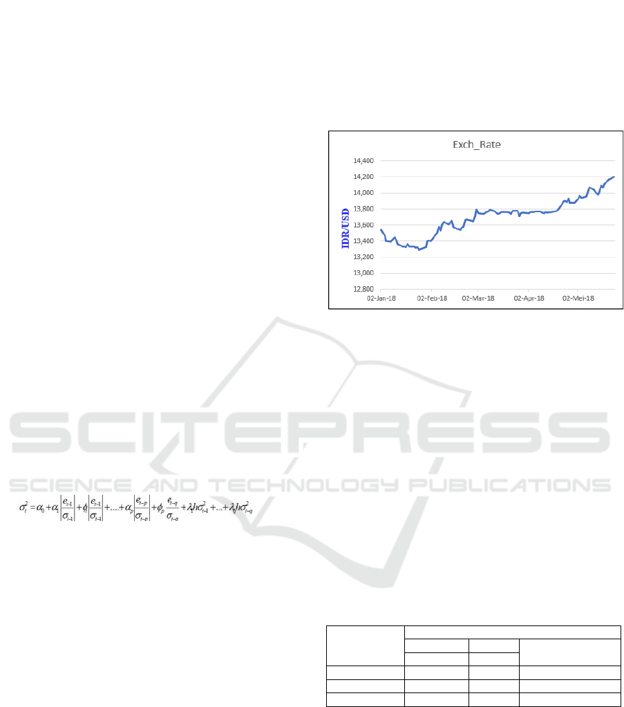
The movement of the IDR to USD exchange rate

from 2 January 2018 to 24 May 2018 is shown in the

following figure.

Figure 1: Movement of the IDR / USD exchange rate

perod Jan 2-May 24, 2018.

The strongest IDR rate occurred on January 25,

2018 with the exchange rate of 13.290, But

unfortunately the next day IDR weakened.

4.2 Testing of Data Stationarity

In the early stages, exchange rate data (KURST) is

transformed into natural logarithmic form with the

aim that the stationary data to the variance. To avoid

spurious regression, the data analyzed must be

stationary (Sumaryanto, 2009). The stationarity test

was done using Augmented Dickey Fuller (ADF)

method to Log KURST (LKURST) and the result

showed in Table 1.

Table 1: Results of the ADF stationarity test at Level.

Stationary test results at Level

-Statistic Prob

Description

0.567448 0.9882

1% level -3.498439 Non-stationary

5% level -2.891234 Non-stationary

10% level -2.582678 Non-stationary

The stationary test results indicate that the data

(LKURST) is not stationary at the level. This can be

seen on the value of t-statistic test which was not

significant, either at alpha 1%, 5%, or 10%.

Therefore it was then tested on the first difference

(DLKURST).

ICEBM Untar 2018 - International Conference on Entrepreneurship and Business Management (ICEBM) Untar

170

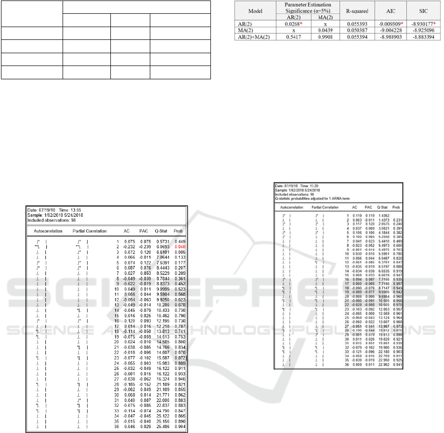
Table 2: ADF test results on First Difference.

Stationary test results at 1

-difference

t-Statistic Prob.* Description

-8.517092 0.0000

1% level -3.499910 Stationary

5% level -2.891871 Stationary

10% level -2.583017 Stationary

The result of the stationary test at the first difference

indicates that the data is stationary. This can be seen

in the significant t-statistical test values at alpha 1%,

5%, or 10%, where the probability is 0.000

4.3 Model Identification

The suitable ARIMA model used can be identified

through ACF and PACF plots of DLKURST as

shown in Figure 2.

Figure 2: First Difference Correlogram.

The ACF and PACF patterns show that the spike

is significant in lag 2, whereas the others are not

significant. Therefore, the tentative ARIMA models

are:

DLKURST = C+ AR(2) (14)

DLKURST = C+ MA(2) (15)

DLKURST = C+ AR(2) +MA(2) (16)

A comparison of the estimation of the three models

is shown in Table 3 below:

Table 3: Comparison of models estimation parameters.

From the comparison of the three models, the

AR(2) model is most statistically significant. In

addition the AR(2) model also has the smallest AIC

and SIC values compared to the other two models.

Based on these considerations, the AR(2) model is

the best model.

4.4 Model Evaluation

The ACF and PACF residual corelogram of the

selected model is shown in the following figure:

Figure 3: Residual corelogram of DLKURST = C + AR

(2).

From ACF and PACF plots of residual values

there is no significant lag up to 36. This showed that

the estimated residual value is random, so the

selected model is already the best model.

4.5 ARCH/GARCH Model

The estimation results in AR(2) above is an ARIMA

model estimation without including ARCH/GARCH

element. So, it must be detected whether the model

contains heteroscedasticity or not. If the model

contains heteroscedasticity problems, the ARIMA

model should be estimated by the ARCH/GARCH

approach.

The test results using Heteroscedasticity Test

White are as follows:

Application of GARCH Model in Forecasting IDR/USD Exchange Rate

171

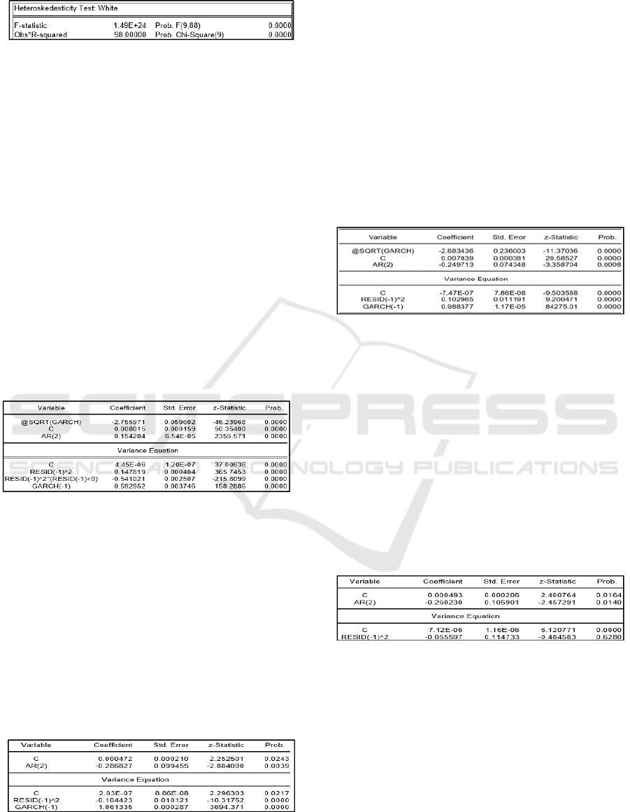
Table 4: Results of Heteroscedasticity Test White.

The result shows the value of Obs * R-squared is

98.0000 while the probability value is 0.0000

(<0.05). This means that Heteroskedasticity Test

White indicates that the data contains

heteroscedasticity problems or there is an ARCH

effect on the estimated model.

4.6 ARCH Model Estimation

Since the estimated model contains ARCH elements,

the next step is to estimate and simulate several

models of variance equations by incorporating the

ARCH element and selecting the best model of the

simulation performed.

4.7 ARCH(1)

The result of ARCH(1) estimation is obtained as

shown in Table 5.

Table 5: Output of ARCH(1) model.

In the variance equation it is shown that the

coefficients of ARCH(1) (at output stated as RESID

(-1)^2) are not statistically significant, which means

there is no volatility in the exchange rate data in the

study period. This means that the exchange rate

residual is not affected by the residuals of the

previous period.

4.8 GARCH(1,1)

The estimation result of GARCH(1,1) model is

shown in the following table:

Table 6: Output of GARCH(1,1).



The variance equation shows that the ARCH(1)

coefficient is statistically significant, which means

there is volatility in the exchange rate data within the

study period and the exchange rate residual is

affected by the residual of the preceding period of

ARCH(1). The GARCH coefficient is also

statistically significant. This means residual

volatility affects the exchange rate.

4.9 ARCH-M

The ARCH-M model was developed using GARCH

elements with additional standard deviation

representations. The regression results are shown in

Table 7.

Table 7: Output of ARCH-M model.

The variance equation shows that the ARCH(1)

coefficient is statistically significant, which means

there is volatility in the exchange rate data. This also

means that the exchange rate residual is influenced

by the residuals of the previous period. The GARCH

coefficient is also statistically significant. This

means residual volatility affects the exchange rate.

4.10 TARCH

In this model, GARCH (1,1) is used with the

addition of threshold. The regression results are

shown in the following Table:

Table 8: TARCH Model Estimation.

The existence of symmetric effects in the model

is shown in the variance equation, ie the RESID (-1)

^ 2 * (RESID (-1) <0) variable. This variable is

statistically significant at alpha 5%, so it can be

concluded that the exchange rate behavior of the

model shows a symmetrical effect.

4.11 Selection of the Best Model

The selection of the best model is based on the

significance of the estimation parameter, the largest

Likelihood Log and the smallest AIC and SIC

criteria. Summaries for these indicators based on the

ICEBM Untar 2018 - International Conference on Entrepreneurship and Business Management (ICEBM) Untar

172

models of variance simulation are shown in table 9.

Table 9: Summary of indicators for best model selection.

Based on the comparison of the indicators, the

GARCH (1,1) model was chosen as the best model.

Furthermore, the best models are then evaluated

with the Residual Normality Test, Residual Random

Test and ARCH Effect Test.

4.12 Testing of Residual Normality

-2.0 -1.5 -1.0 -0.5 0.0 0.5 1.0 1.5 2.0 2.5

Series: Standardized Residuals

Sample 1/03/2018 5/24/2018

Observations 98

Mean 0.024940

Median 0.020504

Maximum 2.546436

Minimum -2.187636

Std. Dev. 0.978798

Skewness 0.172779

Kurtosis 3.007769

Jarque-Bera 0.487839

Probability 0.783551

Figure 4: Residual Normality Test of GARCH (1,1).

The test results show that the Jarque-Bera

Probability value is 0.783551 (> 0.05), means that

the residual is normal and stationary to the variance.

4.13 Testing Residual Randomness

The residual randomness test is performed using

ACF and PACF plots as shown in the following

figure.

Figure 5: The results of residual randomness testing using

ACF and PACF.

ACF and PACF results from residual values

were not significant until lag 36, so it can be

concluded that the residual value of the estimated

GARCH (1,1) model is random.

4.14 ARCH Effect Testing

The ARCH effect test on GARCH (1,1) was

performed by ARCH-LM. Test results are obtained

as follows:

Table 10: Output of Arch Effect Testing.

Based on the calculation, Obs * R-squared value

is 0.5636 with a probability value of 0.5636 (> 0.05).

The ARCH-LM test indicates that the estimated

GARCH (1,1) model is free from the ARCH effect.

4.15 Forecasting

Based on all evaluations that have been done, the

best model with optimal result is GARCH (1,1).

This model can be used to forecast the exchange rate

5-days ahead, that is from 25 May 2018 until 31

May 2018. The forecasting results are obtained as

follows:

Table 11: Forecasting result of IDR against USD.

Date Forecast

25-May-2018 14,065

28-May-2018 14,072

29-May-2018 14,078

30-May-2018 14,084

31-May-2018 14,090

Based on Forecasting using GARCH (1,1), we

obtained MAPE value of 0.201594. This means the

average error is 0.20%. According to Zainun (2010,

16) a model has a very good performance if the

MAPE value is below 10%, and has a good

performance if the MAPE value is between 10% and

20%. With the acquisition of MAPE of 0.20% it can

be said that the GARCH (1.1) model is able to

provide excellent forecasting performance on

IDR/USD exchange rate.

5 CONCLUSION

A study of the volatility of the IDR/USD exchange

rate has been conducted. The results showed that

Application of GARCH Model in Forecasting IDR/USD Exchange Rate

173

there was heteroscedasticity in observation data.

Therefore, based on volatility analysis during the

observation period, the most suitable GARCH model

is GARCH (1,1).

Using the above volatility model, we forecasted

the IDR/USD exchange rate for 5 days from 25 May

2018 to 31 May 2018 and the results are are as

follows 14065, 04072, 14078, 14084 and 14090.

REFERENCES

Adi, U. S., Warsito, B., & Suparti. (2016). Pemodelan

neuro-garch pada return nilai tukar rupiah terhadap

dollar amerika. Jurnal Gaussian, 5, 771–780.

Engle, R. F. (1982). Autoregressive Conditional

Heteroskedasticity twith Estimates of the variance of

United Kingdom Inflation. Econometrica.

Engle, R. F., Lilien, D. M., & Robins., R. P. (1987).

Estimating Time-varying Risk Premia in the Term

Structure: The ARCH-M Model. Econometrica, 55(2),

391–407.

Glosten, L. R., Jaganathan, R., & Runkle, D. E. (1993).

On the relation between the expected value and the

volatility of the nominal excess returns on stocks.

Journal of Finance, 48, 1779–1801.

Hueter, I., & No, W. P. (2016). Latent Instrumental

Variables : A Critical Review. Institute for New

Economic Thinking, (46). Retrieved from

https://www.ineteconomics.org/uploads/papers

Kristjanpoller, W., & Minutolo, M. C. (2016). PT US CR.

Expert Systems With Applications.

https://doi.org/10.1016/j.eswa.2016.08.045

Lin, Z. (2017). Modelling and Forecasting the Stock

Market Volatility of SSE Composite Index Using

GARCH Models. Future Generation Computer

Systems. https://doi.org/10.1016/j.future.2017.08.033

Natsir, K., & Mimi. (2017). Forecasting demand for

Moslem fashion products at DG company in South

Tangerang, Indonesia, (ICEBM), 459–464. Retrieved

from http://icebm.untar.ac.id/index.php/more/

proceedings?id=20

Nelson. Daniel B. (1991). Conditional Heteroscedasticity

in Asset Returns, A New Approach, 347–370.

Pani, A., Desvina, Octaviani, I., & Meijer. (2018).

Penerapan Model ARCH/GARCH untuk Peramalan

Nilai Tukar Petani Ari Pani Desvina 1 , Inggrid

Octaviani Meijer 2. Jurnal Sains Matematika Dan

Statistika, 4(1), 43–54.

Sumaryanto. (2009). Komoditas Pangan Utama Dengan

Model ARCH / GARCH Retail Price Volatility

Analyzes of Some Food Commodities Using Arch /

Garch Model, 135–163.

Tian, S., & Hamori, S. (2015). Modeling interest rate

volatility : A Realized GARCH approach. Journal of

Banking Finance, 61, 158–171.

https://doi.org/10.1016/j.jbankfin.2015.09.008

Widarjono, A. (2002). Aplikasi Model ARCH Kasus

Inflasi di Indonesia. Jurnal Ekonomi Pembangunan.,

71–82.

Zainun, N. Y. B. (2010). Forecasting low-cost housing

demand in Johor Bahru , Malaysia using artificial

neural networks ( ANN ).

Zakoian, J. M. (1990). Threshold Heteroskedastic Model.

Journal of Economic Dynamics and Control.

ICEBM Untar 2018 - International Conference on Entrepreneurship and Business Management (ICEBM) Untar

174