
Lane Effect of Traffic Flow Analysis in India
Tsutomu Tsuboi
Global Business Development Office, Nagoya Electric Works Co., Ltd, 29-1 Mentoku Shinoda, Ama, Japan
Keywords: Traffic Flow Analysis, Road Lanes Effect, Emerging Country Traffic.
Abstract: The aim of this research is to develop quantitative analysis method for emerging countries, especially focusing
on major city in India where they are facing negative impact by transportation such as CO2 emission growth,
many traffic fatalities, large fuel consumption, and air pollution as a result. In this research, we installed more
than ten traffic monitoring traffic counter cameras in Ahmedabad city of Gujarat state of India. The monitoring
cameras detect traffic vehicle and capture several traffic data such as vehicle numbers, vehicle speed, traffic
occupancy, vehicle density, gap length between vehicle to vehicle and so on. And each data is collected by
every minutes per roads. Therefore the collected data becomes more than 432,000 points per months. In order
to analyse the traffic data, author recognize special features of the collected traffic data and the Envelope
Observation (EO) for traffic flow characteristics by measurement data is useful for obtaining traffic flow
equation. The unique feature of emerging counties traffic data is widely spread plots at the traffic basic
characteristics such as traffic density to speed curve and traffic density to traffic volume curve. But there is
clearly boundary line in those curves. Author uses EO analysis to fit traffic flow parameters to these boundary
lines. By defining traffic flow parameters, it is able to obtain the traffic flow value such as free speed traffic
flow, critical traffic volume, and critical traffic density. After obtaining traffic parameters, it is able to create
traffic flow equation for each measured road and even each lane of its road. The uniqueness of this research
is extension of analysis for the road lane effect for the traffic congestion by correlation ratio analysis between
driving lane and passing lane of each road. As the result of this analysis, it becomes clear that congestion
condition of roads makes the different traffic flow characteristics by driving and passing lane. This is the first
time to explain the lane effect for traffic congestion on the basis of the EO method.
1 INTRODUCTION
1.1 Background
This manuscript describes traffic flow analysis
method in emerging county based on one month
probe big data. In general, it is a challenge how to
collect real traffic probe data in emerging country and
how to analyse traffic flow from its data. Author has
a chance to collect total two months traffic probe data
by using traffic monitoring cameras in Ahmedabad
city of Gujarat State in India. This is a part of Japan
International Cooperation Agency or JICA project for
providing traffic information to the drivers in the city
as Indian ITS business since October 2014. In this
project, there are fourteen traffic monitoring cameras
and four electric traffic information sign boards so
called Variable Message Sign (VMS) are installed in
Ahmedabad city. In this paper, one month prove data
in June 2015 is used as lane effective analysis.
In Author’s previous research, we introduced
traffic flow analysis of Ahmedabad city in India and
showed traffic congestion condition by using Envelop
Observation (EO) method in which traffic
characteristics is obtained by utilizing the Envelope
Observation for each measurement traffic data. It is
described in the next section. According the previous
research, speed ratio which is average speed of
vehicles to free flow speed which is obtained from
EO.
The following steps are our traffic flow analysis
in this paper.
At first, we start traffic flow analysis for each
roads by EO method and obtain traffic basic traffic
flow characteristics such as the traffic density (k) to
speed (v) curve (K-V curve). From each K-V curve, it
is able to define free flow speed (v
f
).
As the next step, we calculate a speed ratio (V.R.)
which is the average speed (v
ave
) to the free flow
speed (v
f
). When the critical speed is described as (v
c
),
its value is the half of free flow speed (v
f
) from the
268
Tsuboi, T.
Lane Effect of Traffic Flow Analysis in India.
DOI: 10.5220/0007239302680276
In Proceedings of the 5th International Conference on Vehicle Technology and Intelligent Transport Systems (VEHITS 2019), pages 268-276
ISBN: 978-989-758-374-2
Copyright
c
2019 by SCITEPRESS – Science and Technology Publications, Lda. All rights reserved

theory. Therefore the traffic condition under less than
0.5 V.R. area means congested condition. The V.R.
becomes important parameter for congestion
condition of the roads.
As the third step, we investigate lane effect
against each traffic condition and this analysis is main
study in this paper. In order to analyze the lane effect
to traffic congestion, we compare the variance of
traffic congestion between driving lane and passing
lane. In this study, we have three measured data of the
roads—speed (v), traffic density (k), and traffic
volume (q). For the traffic condition variance, two
value of them are enough for the variance comparison
because there is the relationship among them—
q=k×v. So we chose (v, k) parameter set as
representative traffic characteristics for each lane.
Since the V.R. is congested condition parameter, the
correlation between V.R. and the (v, k) parameter set
of each lane provides lane effectiveness for its traffic
condition.
And finally we show a certain lane effect between
driving lane and passing lane by K-Q curve of each
lane.
This is the first traffic flow analysis in emerging
country in terms of the following features.
Use one month traffic flow big data among 10
locations
Introduce traffic flow equation by EO method
Show lane effectiveness by K-Q curve
characteristics
1.2 Related Study
In terms of traffic analysis, there are new challenges
by using advanced sensing technology such as the
probing data with Global Positioning System (GPS)
in side vehicles. This study is estimation by using
probing vehicle behaviour but this case study is
limited number of probe data and a study in the
advanced country i.e. Italy. For probing technology
based traffic analysis, there are many case studies in
the vehicular ad hoc network (VANET) environment.
These research are useful to estimation traffic safety
application especially in the congested traffic
condition. In VANET environment, the advanced
communication technology is sued such as Dedicated
Short Radio Communication (DSRC), Cellular phone
network like Long term Evolution (LTE), 3G, 4G, 5G
etc. Most of the advanced network communication
technology has just been released in the advanced
countries and will be installed in new manufacturing
vehicles in future.
Therefore the classical traffic monitoring technology
with monitoring cameras is still valid especially for
study of traffic flow analysis in the emerging
countries. In case of traffic analysis in emerging
countries such as India, there are several studies these
days. Goutham.M has proving data analysis at
National Highway in Hyderabad. It shows trend of
traffic condition and comparison with Indian Road
standard IRC-106-1990 but measurement points are
only two Highways and volume is two days with five
CCTVs. In Salim.A et al study, it describes traffic
congestion condition by headway measurement in
Chennai. But measurement point is only one city road
and four days data with one hour for each. It is also
limited measurement data.
2 ENVIRONMENT OF TRAFFIC
DATA MEASUREMENT
2.1 Location
As mentioned in Introduction, the Indian ITS project
has been started since October 2014. The ITS
business operates in Ahmedabad city of Gujarat states
in India, where it is located west region of India and
it has about 8 million population. There are fourteen
traffic monitoring cameras which collect traffic
parameters such as traffic density, traffic volume, and
speed.
The Figure.1 shows total ITS cameras installation
location in the city. The “Cam” in Figure.1 means
Traffic Monitoring Camera and “VMS” means
Various Message Sign board. The main purpose of
VMS is display of traffic condition to drivers after
traffic condition analysis.
Figure 1: Indian ITS system installation location.
2.2 System Configuration
The Indian ITS system has three components—traffic
monitoring camera, traffic information board, traffic
Lane Effect of Traffic Flow Analysis in India
269
management system. The management system is
operated by cloud system through internet access.
The total system configuration is shown in Figure.2.
The traffic data is captured through traffic monitoring
camera and transferred to the data base via Internet
Cloud. After collecting traffic data, the traffic
condition is shown at the VMS as the result of traffic
analysis. The traffic condition information is shown
by the simple three level like conditions such as
heavy, slightly heavy, and smooth.
Figure 2: Indian ITS system configuration.
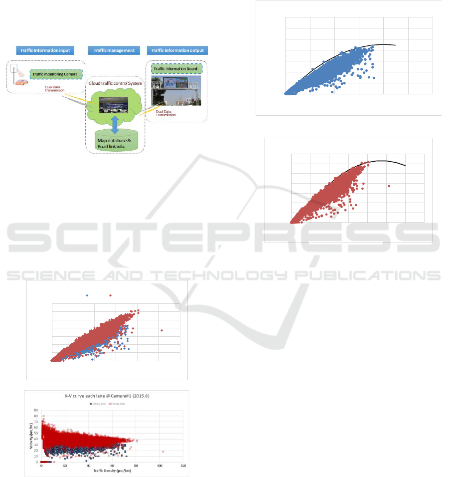
2.3 Traffic Measurement Data
The traffic monitoring cameras measure and collect
the traffic data every minute. Figure.3 (A) and (B)
show an example of K-Q curve and K-V curve of each
lane at Camera#1. The plotted data is measured
during June 2015. The road at Camera#1 has two
lanes for both direction of its roads.
(A) K-Q curve of each lane at Camera#1.
(B) K-V curve of each lane at Camera#1.
Figure 3: Example of traffic characteristics at Camera#1.
According to all measured traffic data, shape of
curve at each location is quite similar configuration.
There is boundary line in each K-Q curve and K-V
curve clearly. There are no measured data out of its
boundary line. Therefore it is able to consider that the
boundary line shows traffic capacity of the road at
least under the measurement time period. Figure.4
(A) and (B) show K-Q curve for driving lane and
passing lane at Camera#1 for example.
(A) K-Q curve of driving lane at Camera#1.
(B) K-Q curve of passing lane at camera#1.
Figure 4: K-Q curve of each lane at Camera#1.
3 ENVELOPE OBSERVATION
METHOD
In this section, it is explained how to obtain the traffic
characteristics by using the Envelop Observation
(EO) method.
3.1 Traffic Flow Equation
From the traffic flow theory, typical K-V and K-Q
curve are described like in Figure.5 (A) and (B). As
we see the boundary line in previous section, the line
is consistent with the envelopment curve. Therefore
when we consider that the boundary line provides the
road capacity of each road, it is able to obtain traffic
parameters from this curve.
0
500
1000
1500
2000
2500
3000
3500
0 20 40 60 80 100 120
Traffic Volume (pcu/hr)
Traffic Density (pcu/km)
K-Q curve each lane @Camera#1 (2015.6)
Driving lane Passing lane
0
500
1000
1500
2000
2500
3000
3500
0 20 40 60 80 100 120
Traffic Volume (pcu/hr)
Traffic Density (pcu/km)
K-Q curve driving lane @Camera#1 (2015.6)
0
500
1000
1500
2000
2500
3000
3500
0 20 40 60 80 100 120 140
Traffic Volume (puc/hr)
Traffic Density (pcu/km)
K-Q curve passing lane @Camera#1 (2015.6)
VEHITS 2019 - 5th International Conference on Vehicle Technology and Intelligent Transport Systems
270
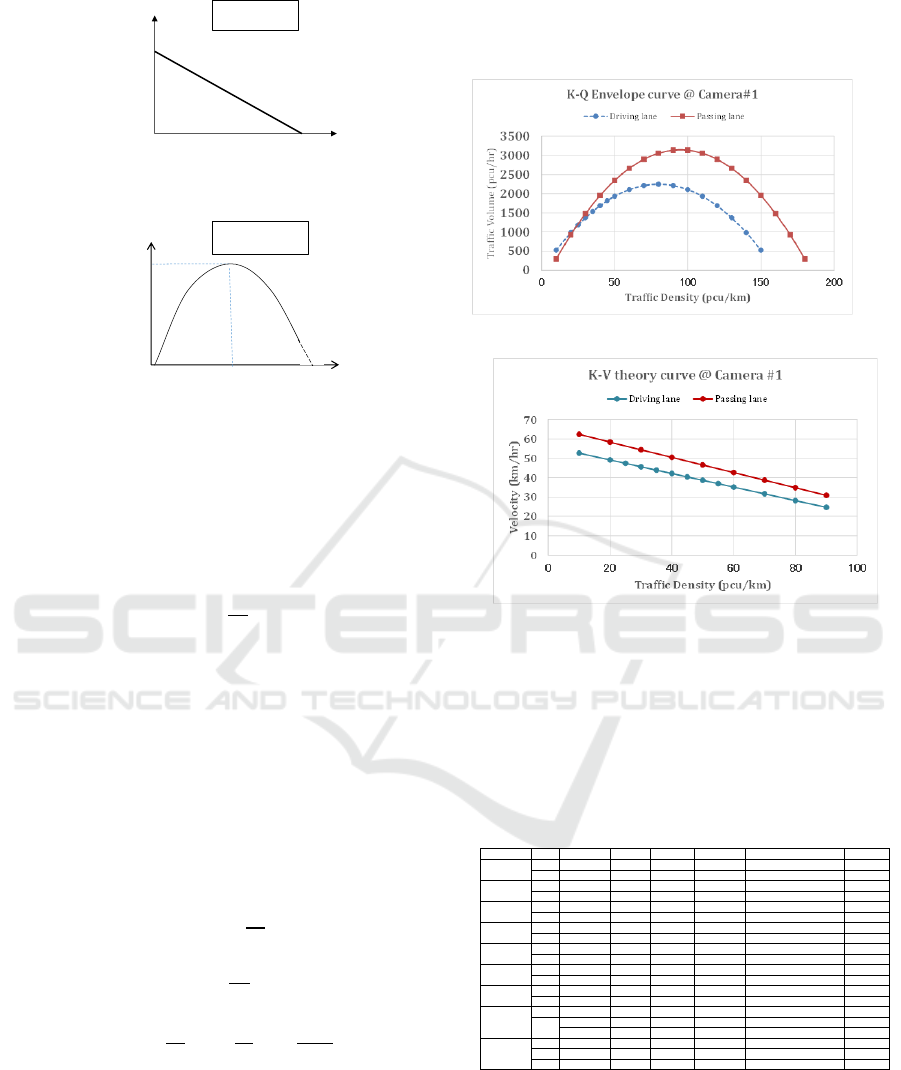
(A) Theoretical K-V curve.
(B) Theoretical K-Q curve.
Figure 5: Traffic Flow Theoretical curve.
The Figure.5 (A) shows one of general K-V curve
which is called Greenshields. It is obtained by
equation (1).
(1)
where (v
f
) is free flow speed and (k
f
) is traffic
density at free flow condition.
From traffic flow continuity of the traffic flow
theory, equation (2) is given.
(2)
where (q) is traffic volume, (k) for traffic density,
(v) for speed.
The following equation (3) is obtained by
eliminating (v) from equation (1) and (2).
(3)
where (k
j
) is jam traffic density and k
j
= 2 k
c
.
3.2 Traffic Flow Characteristics by EO
Method
When we use equation (1) and (3), it is able to obtain
traffic parameters by matching the envelopment line
with its calculated curve by its traffic parameters.
The envelopment curve at Camera#1 in Figure.6 (A)
and (B) as an example.
(A) Envelopment curve of K-Q curve at Camera#1.
(B) Envelopment curve of K-V curve at Camera#1.
Figure 6: Envelopment curve of Traffic Flow
Characteristics of Camera#1.
By using EO method for all measurement traffic data in
Ahmedabad, Table 1 shows the summary of the analysis
result at each location.
Table 1: Traffic Parameters at each Location by EO
Method.
The data of Camera#5 and #9 are eliminated
because of measurement trouble. The number of lane
of Camera#1 to #7 and VMS#3 is two lane and that
of Camera#8 and #10 is three lanes for each side of
the road.
vf
kj
0
k-v curve
k
v
Traffic density
velocity
kj
0
k
q
qc
kc
k-q curve
Traffic density
Traffic volume
Location Lane
v
f
/kj kc(pcu/km) qc(pcu/hr) vc (km/hr) K -Q curve Formula vf (km/hr)
DL 0.35156 80 2250 28.13 -0.3516(k-80)^2+2250 56.3
PL 0.34903 95 3150 33.16 -0.3951(k-95)^2+3150 66.3
DL 0.17355 110 2100 19.09 -0.1736(k-110)^2+2100 38.2
PL 0.22222 120 3200 26.67 -0.2222(k-120)^2+3200 53.3
DL 0.24377 95 2200 23.16 -0.2438(k-95)^2+2200 46.3
PL 0.26446 110 3200 29.09 -0.2645(k-110)^2+3200 58.2
DL 0.39446 85 2850 33.53 -0.3945k-85)^2+2850 67.1
PL 0.35000 100 3500 35.00 -0.3500(k-100)^2+3500 70.0
DL 0.21607 95 1950 20.53 -0.2161(k-90)^2+1950 41.1
PL 0.28733 115 3800 33.04 -0.2873(k-115)^2+3800 66.1
DL 0.24793 110 3000 27.27 -0.2479(k-110)^2+3000 54.5
PL 0.28099 110 3400 30.91 -0.2810(k-110)^2+3400 61.8
DL 0.24306 120 3500 29.17 -0.2431(k-120)^2+3500 58.3
PL 0.28099 110 3400 30.91 -0.2810(k-110)^2+3400 61.8
DL 0.25620 110 3,100 28.18
-0.2562(k -110)^2+3100 56.4
1PL 0.35000 100 3,500 35.00
-0.3500(k -100)^2+3500 70.0
2PL 0.41975 90 3,400 37.78
-0.4198(k-9 0)^2+3400 75.6
DL 0.28906 80 1850 23.13 -0.2891(k-80)^2+1850 46.3
1PL 0.37500 80 2400 30.00 -0.3750(k-80)^2+2400 60.0
2PL 0.42857 70 2100 30.00 -0.4286(k-70)^2+2100 60.0
DL: Driving Lane, PL: Passing Lane, 1PL: 1st Passing Lane, 2PL: 2nd Passing Lane
VMS#3
Cam#8
Cam#10
Cam#1
Cam#2
Cam#3
Cam#4
Cam#6
Cam#7
Lane Effect of Traffic Flow Analysis in India
271
4 LANE EFFECT ANALYSIS
4.1 Congestion and Speed Ratio
In the previous research, it is concluded that there is
strong relationship between traffic congestion and
speed ratio (V.R.) which is average speed (v
ave
) to free
flow speed (v
f
). When k=k
c
=k
j
/2 in equation (1),
v=1/2v
f
. And the critical traffic volume (q
c
) is
obtained when k=k
j
/2. The road condition over (q
c
)
becomes congestion condition which is shown in
Figure.7.
Figure 7: Traffic density and Traffic Volume relationship.
The Figure.8 shows the summary of V.R. of each
location. In Figure.8, DL means the driving lane, 1PL
is the first passing lane, and 2PL is the second passing
lane.
Figure 8: Speed ratio (V.R.) at each Location.
As it is shown in Figure.8, the condition at
Camera#2 is congested of both the driving lane and
passing lane. The driving lane condition at Camera#3
is also congested.
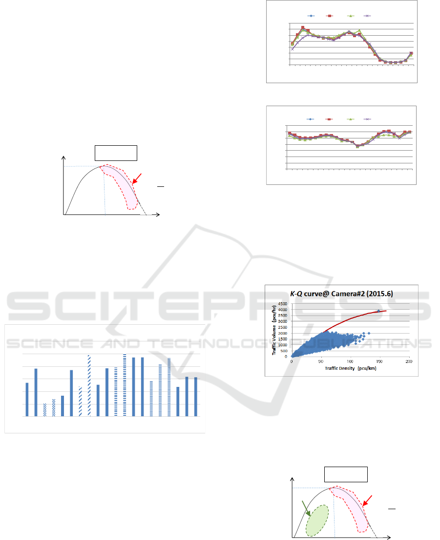
In order to understand the condition at Camera#2,
the time zone based traffic volume and speed at
Camera#2 are shown in Figure.9. In Figure.9 (A), we
see two heavy traffic volume time zones which are
around 9:00 am and 8:00 pm.
(A) Time zone base Traffic Volume at Camera#2.
(B) Time zone base Speed at Camera#2.
Figure 9: Time zone traffic characteristics at Camera#2.
As for the time zone based speed in Figure.9 (B),
the speed at 8:00 pm drops down under 20km/hr
which means the traffic condition is congested.
The actual K-Q curve from the measured data at
Camera#2 is shown in Figure.10.
Figure 10: The Actual K-Q curve from the measured data at
Camera#2.
According to Figure.10, there is no measured data
over the critical traffic volume. This shows there is
another new congested area except the area with over
traffic critical volume. Figure.11 shows this condition.
Figure 11: New congested area in Indian traffic.
kj
0
k
q
qc
kc
k-q curve
Traffic density
Traffic volume
2
j
c
k
k
Congested condition
DL
1PL
DL
1PL
DL
1PL
DL
1PL
DL
1PL
DL
1PL
DL
1PL
DL
1PL
2PL
DL
1PL
2PL
0.40
0.45
0.50
0.55
0.60
0.65
0.70
Velocty Ratio Comparison
Cam#1 Cam#2
Cam#3
Cam#4 Cam#6
Cam#7 VMS#3 Cam#8
Cam#10
DL: Driving lane 1PL: 1st Passing lane 2PL: 2nd Passing lane
0
200
400
600
800
1000
1200
1400
7 8 9 10 111213 14 15 1617 18 192021 22 23 0 1 2 3 4 5 6
Traffic Volume
(pcu/hr)
Time Zone
Traffic Volume @ Camera#2 (2015.6)
Qave Qweek Qsa Qsu
0
5
10
15
20
25
30
35
7 8 9 10 11 12 1314 1516 1718 1920212223 0 1 2 3 4 5 6
Velocity
(km/hr)
Time Zone
Velocity @ Camera#2 (2015.6)
Vave Vweek Vsa Vsu
kj
0
k
q
qc
kc
k-q curve
Traffic density
Traffic volume
2
j
c
k
k
Congested condition
New
Congested
area
VEHITS 2019 - 5th International Conference on Vehicle Technology and Intelligent Transport Systems
272
The Figure.11 explains that the value of traffic
volume does not always provides the traffic
congestion condition, which we have already seen the
traffic condition around 9:00 am in Figure.9 (A).
Therefore it is able to say that V.R. is valid parameter
which defines traffic congestion.
4.2 Lane Effect
As it is shown in Figure.8, the traffic conditions of
each road and each lane are different. In order to
understand their lane effect for traffic flow, we
calculate the variance of measurement data set with
the elements of traffic density (k) and Speed (v). Here
we define data set of the driving lane is DL(k, v) and
the passing lane data set is PL(k, v). The correction
ration between driving lane (DL) and passing lane
(PL) are shown in Table 2. The data set of the 1st
passing lane is (1PL) and the 2nd passing lane is
(2PL).
Table 2: Correlation Ratio at Each Location.
According Table 2, the value of correlation ratio
at Camera#2 is highest score, which means the traffic
condition of the driving lane and the passing lane are
both congested. This is what it has been already
shown that the traffic condition at Camera#2 is most
congested (refer to Figure.8 (B)).
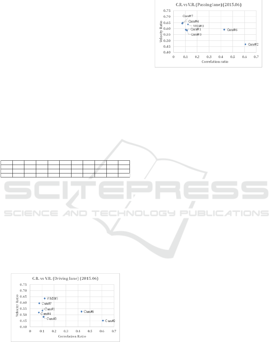
4.3 Correlation Ratio and Speed Ratio
In this section, we investigate relationship between
correlation ratio (C.R.) and speed ratio (V.R.).
Figure.12 shows the relationship for each lane.
(A) C.R. vs V.R in driving lane
(B) C.R. vs V.R in passing lane
Figure 12: Relationship between C.R. and V.R
From Figure.12, the lower speed ratio which
means traffic congestion condition, the higher
correlation ratio which means different traffic
characteristics between driving lane and passing lane.
Figure.13 shows K-Q envelopment curve at VMS#3,
Camera#6 and Camera#2.
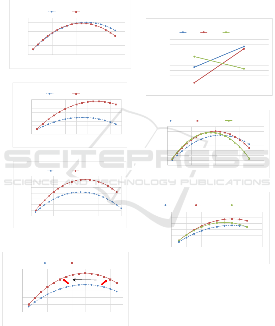
4.4 Comparison Traffic Characteristics
In previous section C, K-Q characteristics curve at
VMS#3, Camera#6 and Camera#2 is described. As it
is shown in Figure.9, traffic condition atVMS#3 is
smooth flow compared with that of camera#2 and
Camera#6 is middle.
From Figure.13, it is clear different traffic
characteristics between the driving lane and the
passing lane based on congestion condition.
For the summary for lane effect to traffic
characteristics, it is possible to the following
conclusion.
i) In free flow condition: there is no particular
different between driving lane and passing lane
(Figure.13 (A))
ii) Medium congested condition: there is a certain
different especially in low traffic density
condition (Figure.13 (B))
iii) Congested condition: there is big difference
between driving lane and passing lane (Figure.13
(C))
The above summary is illustrated in Figure.14.
The different characteristics between driving lane and
passing lane becomes clearer according to congestion
level of the road. From the beginning of traffic
congestion, traffic volume difference becomes bigger
at lower traffic density condition (A point in
Figure.14). Then when traffic condition becomes
more congested, traffic volume difference at higher
traffic density becomes bigger (point B in Figure.14).
Cam#1 Cam#2 Cam#3 Cam#4 Cam#6 Cam#7 Cam#8 Cam#10 Cam#10 VMS#3
DL-PL 0.103 0.608 0.113 0.074 0.429 0.077 0.073 0.153 0.153 0.122
1PL-2PL 0.013 0.144 0.144
DL-2PL 0.114 0.067 0.067
Lane Effect of Traffic Flow Analysis in India
273
In terms of lane effect research, Uchida.H
announced highway level analysis in Japan. But this
is based on simulation model analysis and lane effect
shows up in high traffic density area.
(A) K-Q characteristics curve at VMS#3.
(B) K-Q characteristics curve at Camera#6.
(C) K-Q characteristics curve at Camera#2.
Figure 13: K-Q characteristics curve at typical location.
Figure 14: Lane Effect in K-Q envelopment curve.
4.5 Three Lane Analysis
In case of three lane case study, we only have data of
Camera#8 and #10. Figure.15. The correlation ratio
and vehicle ratio relationship, K-Q envelopment
curve at Camera#8 and #9 are shown in Figure.15.
(A) Correlation ratio at Camera#8 and #10
(B) K-Q characteristics curve at Camera#8.
(C) K-Q characteristics at Camera#10.
Figure 15: Three lane traffic characteristics Comparison.
There is no significant characteristics difference
among three lanes because correlation ratio is small
and traffic condition is relatively smooth.
0
500
1000
1500
2000
2500
3000
3500
4000
0 50 100 150 200
Traffic Volume (pcu/hr)
Traffic Density (pcu/km)
K-Q Envelope curve @ VMS#3 (2015.6)
Driving lane Passing lane
0
500
1000
1500
2000
2500
3000
3500
4000
0 20 40 60 80 100 120 140 160
Traffic Volume (pcu/hr)
Traffic Density (pcu/km)
K-Q Envelop curve @ Camera#6 (2015.6)
Driving lane Passing lane
0
500
1000
1500
2000
2500
3000
3500
0 50 100 150 200
Trffic Volume (puc/hr)
Traffic Density (pcu/km)
K-Q Envelop curve @ Camera#2 (2015.6)
Driving lane Passing lane
0
500
1000
1500
2000
2500
3000
0 20 40 60 80 100 120 140 160
Traffic Volume (pcu/hr)
Traffic Density (pcu/km)
K-Q Envelop curve
Driving lane Passing lane
A
B
0.000
0.020
0.040
0.060
0.080
0.100
0.120
0.140
0.160
0.180
Cam#8 Cam#10
Correlation ratio
Correlation ratio of 3 lanes road
DL-1PL 1PL-2PL DL-2PL
0
500
1000
1500
2000
2500
3000
3500
4000
0 50 100 150 200
Traffic Volume (pcu/hr)
Traffic Density (pcu/km)
K-Q Envelop curve @ Camera #8 (2015.6)
Driving lane 1st Passing lane 2nd Passing lane
0
500
1000
1500
2000
2500
3000
0 20 40 60 80 100 120
Traffic Volume (pcu/hr)
Traffic Density (pcu/km)
K-Q Envelop curve @ Camera#10 (2015.6)
Driving lane 1st Passing lane 2nd Passing lane
VEHITS 2019 - 5th International Conference on Vehicle Technology and Intelligent Transport Systems
274
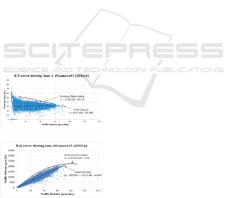
5 DISCUSSION
In this section, it is more detail discussion about the
Envelop Observation method. The Figure.16 shows
K-V curve at driving lane of Camera#1 with
approximate line by Envelop Observation method
and Least Square method. The Least Square method
is generally used in Statics Analysis for understand
the trend of measurement data. From Figure.16, the
equation by Least Square method is right rising curve,
which does not follow the traffic flow theory. On the
other hand, the equation by Envelop Observation
method is right downward curve and follows the
traffic flow theory. In this example, the Envelop
Observation method shows the traffic flow limitation
of each road.
In case of K-Q curve at Camera #1, the traffic flow
characteristics is shown in Figure.17. The Envelop
Observation equation of K-Q curve is q= - 0.3516(k –
80)2+2250. Therefore the jam density k
j
=160. From
equation (3), the free speed v
f
=56.25. When the Least
Square equation of k-q curve from Figure.17, q= -
0.022k
2
+31.213k+4.689=-0.022(k-
709.4)
2
+503233.2. The jam density k
j
=1418.772.
Then free speed v
f
= 31.21. It does not match with v
f
of Figure.16.
As the result, it is able to say that the Least Square
method shows the trend of traffic measurement data
but it does not provide the traffic parameter data such
as jam density and free speed.
Figure 16: K-V curve driving lane at Camera#1.
Figure 17: K-Q curve driving lane at Camera#1.
6 CONCLUSIONS
Author introduce Envelop Observation (EO) method
for emerging country traffic flow study based on one
month big data of traffic at a city in India. By using
EO method, it is able to get traffic flow parameters
such as free flow speed. From the free flow speed, we
are able to get Speed Ratio (average speed to free flow
speed) as indication of traffic congestion level. After
validation of EO method and Speed Ratio is
confirmed, we look into traffic flow difference for
driving lane and passing lane as a lane effect by
correlation ratio between traffic flow condition of
driving lane and passing lane. And we reach the
following conclusion for traffic flow lane effect.
1) Under free flow condition: There is no different
about traffic flow condition. We are able to confirm
this by K-Q curve characteristics.
2) Under light congested flow condition: There is
traffic flow volume different between at driving lane
and passing lane. The traffic volume at passing lane
is larger than that of driving lane, especially high
traffic density condition.
3) Under congested flow condition: There is clear
difference in traffic volume not only at high traffic
density condition but also small traffic density
condition.
In this research, we show that EO analysis method
and correlation ratio comparison for multiple lane
road is useful for the analysis of traffic flow
condition. So we consider this analysis method to
other case study such as time zone base, season base,
and location base in future.
ACKNOWLEDGEMENTS
This research is a part of SATREPS (Science and
Technology Research Partnership for Sustainable
Development) program 2016 (ID: 16667556).
Special appreciation to Mr.Kikuchi.C and
Mr.Mallesh.B of Zero-Sum ITS India for providing
traffic data in Ahmedabad.
REFERENCES
Tsuboi.T, Komori.H, Tatsugami.Y., 2016. Smart Mobility
by Visualization with VMS under ITS project with PPP
business model in India, Japan Society of Traffic
Engineers, vol.51, No.4, pp.28-32.
Lane Effect of Traffic Flow Analysis in India
275

Tsuboi.T, Yoshikawa.Y., 2017. Traffic Flow Analysis in
Emerging Country (India), CODATU XVII.
Tsuboi.T, Oguri.K., 2016. Traffic Flow Analysis in
Emerging Country, Information Processing Society of
Japan Journal, Vol.57, No.4, pp.1284-1289
Tsuboi.T, Oguri,.K., 2016. Analysis of Traffic Flow and
Traffic Congestion in Emerging Country, Information
Processing Society of Japan Journal, Vol.57, No.12,
pp.2819-2826.
Carli.R, Dotoli.M, Epicoco.N, 2017. Monitoring traffic
congestion in urban areas through probe vehicle: A
case study analysis, Wiley Online Library,
https://onlinelibrary.wiley.com/doi/pdf/10.1002/itl2.5
Ahmed.S.H, et al, 2016. Controlled data and Interest
Evaluation in Viheicular Named data Networks, IEEE
Trans Vehicle Technology, 65(6), pp.395-3963.
Goutham.M, Chanda.B., 2014. Introduction to the selection
of corridor and requirement, implementation of IHVS
(Intelligent Vehicle Highway System) In Hyderabad,
International Journal of Modern Engineering Research,
Vol.4, Iss.7, pp.49-54.
Salim.A, Vanajakshi.L, Subramanian.C., 2010. Estimation
of Average Space Headway under Heterogeneous
Traffic Conditions, International of Recent Trends in
Engineering and Technology, Vol. 3, No. 5.
Ohashi.K,, Yanagisaa,.Y, Sakagishi.S., etal., Traffic System
Engineering, Corona Publishing Co. Ltd., p.94.
Greenshields.B.D., 1934. A Study of Traffic Capaci,
Proc.H.R.B., 14, pp.448‐477.
Uchida.H., Arai,.S. 2005. Influence of Driver’s Speed
Selection and Rearward View on Multi-lane Traffic
Flow, The 23rd Annual Conference of Japanese Society
for Artificial Intelligence.
VEHITS 2019 - 5th International Conference on Vehicle Technology and Intelligent Transport Systems
276
