
Spectral Multi-Dimensional Scaling using Biharmonic Distance
Jun Yang
1
, Alexander Jesuorobo Obaseki
1
and Jim X Chen
2
1
School of Electronic and Information Engineering, Lanzhou Jiaotong University, Lanzhou, Gansu 730070, China
2
Department of Computer Science, George Mason University, Fairfax, VA 22030-4444, U.S.A.
Keywords: Canonical Forms, Laplace-Beltrami Operator, Biharmonic Distance, Spectral Multidimensional Scaling
(S-MDS).
Abstract: The spectral property of the Laplace-Beltrami operator has become relevant in shape analysis. One of the
numerous methods that employ the strength of Laplace-Beltrami operator eigen-properties in shape analysis
is the spectral multidimensional scaling which maps the MDS problem into the eigenspace of its Laplace-
Beltrami operator. Using the biharmonic distance we show a further reduction in the complexities of the
canonical form of shapes making similarities and dissimilarities of isometric shapes more efficiently
computed. With the theoretical sound biharmonic distance we embed the intrinsic property of a given shape
into a Euclidean metric space. Utilizing the farthest-point sampling strategy to select a subset of sampled
points, we combine the potency of the spectral multidimensional scaling with global awareness of the
biharmonic distance operator to propose an approach which embeds canonical forms images that shows
further “resemblance” between isometric shapes. Experimental result shows an efficient and effective
approximation with both distinctive local features and yet a robust global property of both the model and
probe shapes. In comparison to a recent state-of-the-art work, the proposed approach can achieve
comparable or even better results and have practical computational efficiency as well.
1 INTRODUCTION
The problem of shape matching has become an
important research problem and a fundamental task
in a wide range of geometric applications including
but not limited to computer vision (Vankaick et al.,
2011), texture mapping (Sumner and Popovic, 2004),
mesh deformation (Kreavoy et al., 2003), morphing
(Alexa, 2002), and shape retrieval (Jain and Zhang,
2006).This problem can be defined as finding the
(dis)similarities between objects represented by
point clouds or triangle meshes, say two different
poses of the same object. Such a problem can be
reduced to establishing a correspondence between
two set of the mesh vertices, that is to say
establishing a meaningful mapping between them.
This mapping is either between coarse sets of feature
points selected on the meshes, or a dense continuous
one that involve all points on the two shapes.
The basic question is finding an effective, yet
accurate way to quantify the similarity between a
given reference surface; “the model” and some other
version (articulated) of the model; “the probe”. An
extrinsic property characterizes how a particular
surface is immersed into the ambient (Euclidean)
space and thus changes as the surface undergoes
transformations. Such a metric is not ideal to capture
distinction between shapes as they are significant
disparities between the extrinsic attributes of a shape
and its articulated version. A deformation that
preserves the intrinsic structure of the surface is
called an “isometry” (Bronstein et al., 2006).Thus
defining a computable deformation-invariant
measure of intrinsic similarity between the surfaces
becomes the task at hand.
2 RELATED WORK
Manifold learning refers to the process of non-linear
dimensionality reduction of data. When target space
of reduction (embedding) is Euclidean the procedure
is also known as flattening and the output is called
“canonical forms” (CF). Multi-Dimensional Scaling
(MDS) is a class of computationally efficient
methods used for embedding a canonical form.
One of the earliest methods finds a uniform
parameterization for convoluted surfaces that is
usually a priori in a more general surface matching
procedure (Schwartz et al. 1989). This result led to
Yang, J., Obaseki, A. and Chen, J.
Spectral Multi-Dimensional Scaling using Biharmonic Distance.
DOI: 10.5220/0007242901610168
In Proceedings of the 14th International Joint Conference on Computer Vision, Imaging and Computer Graphics Theory and Applications (VISIGRAPP 2019), pages 161-168
ISBN: 978-989-758-354-4
Copyright
c
2019 by SCITEPRESS – Science and Technology Publications, Lda. All rights reser ved
161

emergence of many efficient flattening algorithms
like in texture mapping (Zigelman et al., 2002), higher
dimensional Euclidean space embedding (Elad and
Kimmel, 2003) that captures the intrinsic geometric
structure of isometric surfaces and a more
generalized framework (Bronstein et al., 2006) that
uses Gromov-Hausdroff distance (Gromov, 1981) to
compute partial embedding distance for both full and
partial surface matching. The key to using MDS
algorithm for embedding is to obtain intrinsic
representation of the underlying surface which is
invariant to inelastic bending, and then interpolate
this representation to embed the surface in a new
ambient space such that the intrinsic geometry of the
surface is translated into its extrinsic geometry in the
new space. Conventionally, a set of inter-geodesic
distance between pairs of all surface points is used
as input. This approach though efficient, is
computationally expensive as the complexity
requirement in storing all pairwise distance is
quadratic in the number of data points which is
restrictive in shapes with substantial amount of
vertices.
In the last decade, a major breakthrough in the
eigenspace of the mesh Laplacian (Wolter et al., 2006)
has been exploited in variety of forms. Isospectral
properties of the eigenvectors know from linear
algebra provided theoretical foundations that have
been extended to correspondence between 3D
surfaces. Jain et al. (Jain et al., 2011) transformed 3D
meshes into the spectral domain, based on geodesic
affinities, and then matched the spectral embeddings
of the eigenvectors with respect to uniform scaling
and rigid-body transformation. Kim et al. (Kim et al.,
2011) approached the problem by blending a
collection of weighted low dimensional conformal
maps. The multi-scale geometry aware properties of
the Laplace Beltrami operator (LBO) are utilized to
infer and manipulate point-to-point maps between
shapes (Ovsjanikov et al., 2012). Rustamov
(Rustamov, 2007) introduced a deformation invariant
representation of surfaces similar to canonical forms
which is based on combining eigenvalues and
eigenvectors of LBO instead of geodesic distance. A
LBO decomposition method is exploited to construct
diffusion maps (Coifman and Lafon, 2006).
Descriptors like Heat kernel signature (Sun et al.,
2009), wave kernel signature (Aubry et al., 2011) are
all based on eigenfunctions of the LBO.
Similar to our approach, Aflalo et al. (Aflalo and
Kimmel, 2013) extracted the spectral data from the
LBO of pairwise geodesic distance of sampled
points, and then embedded the data into a low-
dimensional Euclidean space. Computed a small
fraction of the pairwise distances that was projected
onto the leading eigenfunctions of the LBO, thus,
efficiently reduced both the time and space
complexities of the flattening procedure. It seems
that they overcame a great amount of complexities,
however, the question of its reliance on geodesic
distance which has weak “global–awareness” and
significantly large topological sensitivity is a major
drawback to this approach.
In this paper, we argue that biharmonic distance
(Lipman et al., 2010) can serve as an efficient yet
accurate distance operator. The measure of
biharmonic distance on shapes are smooth functions,
thus are well suited for compact spectral
representation, and as such allow us to apply this
theoretically sound distance operator in a spectral
sense. Biharmonic distance is a metric structure that
is related to diffusion distance and commute-time
distance (Fouss et al., 2007; Yen et al., 2007) with a
slight modification in the eigenvalue normalization.
Our motivation to use this distance operator is based
on the fact that it finds a good trade-off between
local and global properties of the shape. Here, the
eigenvalue normalization decays slow enough to
get good local properties around source points and
fast enough to be globally aware of shape in far
areas.
3 COMPUTING BIHARMONIC
DISTANCE
Biharmonic distance is a distance operator endowed
with the fundamental properties required for shape
analysis, such as isometric invariant, practically
efficient, parameter-free, insensitive to noise and
topology, etc.
Let us consider a Riemannian manifold M
equipped with a metric G. The metric G induces a
Laplace-Beltrami operator (LBO) denoted by
G
Δ
.
The LBO is self-adjoint and defines a set of
functions called eigenfunctions, denoted by
i
φ
, such
that
iii
φ
λ
φ
Δ=
, where
i
λ
is the eigenvalue
associated with
i
φ
at vertex i.
Biharmonic distance operator is similar to
diffusion distance and the commute-time distance,
however there is slight modification on the
eigenvalue normalization. This normalization
is based on a kernel, which is Green’s function of
the biharmonic differential equation. In the
continuous setting, the squared distance is defined
GRAPP 2019 - 14th International Conference on Computer Graphics Theory and Applications
162

by using the eigenfunctions of the LBO (Lipman et
al., 2010):
2
2
2
1
(() ())
(, )
ii
B
i
i
x
y
dxy
φφ
λ
∞
=
−
=
(1)
The quadratic normalization as shown in the Eq.
(1) provides a good trade-off in the sense that it
decays slow enough to get good local properties
around the point and fast enough to be shape aware
in distance areas. The trade-off is intimately related
to the biharmonic equation. Expanding Eq. (1) we
obtain:
22
2
22 2
11 1
|()| |()| ()()
(, ) 2
(,) (,) 2 (,)
ii ii
B
ii i
ii i
BB B
x
yxy
dxy
gxx gyy gxy
φφ φφ
λλ λ
∞∞ ∞
== =
=+−
=+−
(2)
Using the Green’s function of the biharmonic
operator:
2
1
() ()
(, )
ii
B
k
i
x
y
gxy
φφ
λ
∞
=
=
(3)
The above equation satisfies the relation
2
()
(, ) () ()Δ=
xB
g
xyf ydy f x (4)
for “smooth enough” (Coifman and Lafon, 2006).
From Eq. (3), a discrete construction based on
the discrete Green’s function
of the Bi-Laplacian
is derived from the well-known cotangent formula
discretization of the Laplace-Beltrami differential
operator on shapes (Grinspun et al., 2006; Meyer et al.,
2003).
()()
()
1
cot cot
∈
Δ= + −
ei i
iijijij
jN
i
uu
A
αβ
(5)
where
Δ
i
, denotes the discrete Laplacian evaluated
at vertex i (for
1, 2, , ,= iN
N is the number of
vertices),
i
A
is the Voronoi area at
th
i
shape vertex
(Grinspun et al., 2006) and angles
ij
α
,
ij
β
are the two
angles supporting the edge connecting vertices i and
j respectively.
Having discretized the Laplacian, the Green’s
function of the Bi-Laplacian,
×
∈
NN
d
g
is defined
by discretizing the relation in Eq. (4) to obtain:
2
=
dd
LgAf f
(6)
where
1×
∈
N
f
is an arbitrary vector in the image
of
2
d
L
. (See (Meyer et al., 2003) for prove).
Finally, having obtained
d
g
, the biharmonic
distance on the shape is defined from Eq. (3):
()
() ( ) ( )
2
,,,-2,=+
Bi j d d d
dvv gii g jj gij
(7)
4 SPECTRAL
MULTIDIMENSIONAL
SCALING
Let us consider the shape correspondence problem
that involves searching for the best point to point
matching of two given shapes, S and Q. The earliest
method of using multidimensional scaling (MDS) to
compute such an assignment was proposed by (Elad
and Kimmel, 2003). There, the pairwise geodesic
distances between all points on a 3D shape was
mapped to a simpler 3D Euclidean distance.
The spectral multidimensional scaling (Aflalo and
Kimmel, 2013) uses the fact that point to point
correspondence between two shapes induces a map
between the natural eigenspaces of the shapes, thus,
project the MDS problem into the data’s spectral
domain extracted from its Laplace-Beltrami
operator. In this framework, truncated
eigenfunctions were used to faithfully approximate
correspondence between the shapes. We will go
forward to briefly explain this approach.
Consider a manifold M, with n points
{
}
i
V
, P is
a subset of
{
}
i
V
such that
=≤
s
P
pn
, and a
smooth function f is defined on
{
}
,=∈
Pp
VVpP.
Computing a smooth interpolation function requires
firstly constructing a continuous function h such that
() ()
,=∀∈
pp
f
VfVpP. Then a smooth function
measure the smoothness of such a function, say up
to L
2
norm as
()
2
2
,=∇ =Δ
nn
smooth
MM
Ef fda ffda
.
The problem of smooth interpolation could be
rewritten as
()
() ()
:
min s.t. ,
→
==∀∈
smooth p p
hM
Eh hVfVpP
. Then
we have
2
2
,∇=Δ
nn
MM
f
da h h da
. Thus the
interpolation problem could be written as:
() ()
:
min , s.t. ,
→
Δ=∀∈
n
pp
M
hM
hh da hV f V p P
(8)
In a discrete setting the problem in Eq. (8) above
can be rewritten as
T
min s.t. =
x
x
Wx Bx f
(9)
There the matrix B, represents a projection on the
basis vectors
, ∀∈
p
epP
, W is the conformal
discrete Laplacian without the area normalization
and f is the sampled vector
()
p
f
V . Their novel
Spectral Multi-Dimensional Scaling using Biharmonic Distance
163

technique was to introduce
f
, the spectral
projection of f (the eigenvectors of the LBO
{}
1=
k
i
i
φ
)
as
1
,
=
== =
k
ii
i
xf f
φφ
Φα
, where
Δ=
ii
φ
λ
φ
.
Note that
Φ
represents the matrix of eigenfunctions
whose
th
i
column is
i
φ
such that
,=
ii
f
α
φ
. Thus
Eq. (9) is approximated as
TT
min s.t.
k
WBf
α
αΦ Φα Φα
∈
=
(10)
Since
T
= W
ΛΦ Φ
, where
Λ
is the diagonal
matrix whose elements
ii
λ
are the corresponding
eigenvalues of linear transformation of the LBO L
d
.
Substituting
Λ
and adding the constraint check in
the target function the solution is rewritten as
()
1
TT TT
2
−
=+ + =
B
BBfMf
αμΛμΦ Φ Φ
(11)
The discretized smooth energy of the matrix D is
given by
()
()( )
TT
=+
smooth
EDtraceDWDAtraceDWDA
(12)
While the spectral projection of D
onto
Φ
, is
denoted in matrix form by
T
=D
ΦαΦ
(13)
Substituting D into Eq. (12) we obtain the smooth
spectral interpolation as
() ()
()
()
()
TT
2
T
,
min
,
×
∈
∈
++
−
kk
ij
ij
ij I
F
trace trace
DV V
α
αΛα αΛα
μΦαΦ
(14)
where
F
is the Frobenius norm, k is the number
of eigenfunctions.
A less accurate but efficient way to obtain an
approximation of the spectral interpolation matrix
α
is given as
T
=
M
FM
α
(15)
This is obtained by interpolating the column
vectors f and
i
φ
. Note in the above equation F is
simply a matrix of the sample points V
i
, V
j
and M
represents a matrix such that
=
M
f
α
from Eq. (11).
5 SPECTRAL MDS USING
BIHARMONIC DISTANCE
Following the method of spectral multidimensional
scaling, we apply biharmonic distance to compute
the canonical forms for non-rigid shapes. Given M, a
metric space endowed with a metric
:DM M×→
, and
{
}
12
,,,
n
VVV V=
a finite
set of elements in M, the multidimensional scaling of
V in
k
involves finding a set of points
{
}
12
,,,
n
XXX X=
in
k
whose pairwise
Euclidean distances
()
2
,
ij i j
dX X X X=−
are as
close as possible to
()
,
ij
DV V for all (i, j).
For such an embedding, a family of MDS known
as classical scaling can be realized by the following
minimization program
T
1
min
2
X
F
X
XJDJ−
, where
D
represents a matrix defined by
()
2
,
ij i j
DDVV=
and
T
1
11
nnn
JI
n
=−
, or
1
ij ij
J
n
δ
=−
.
Using Classical scaling in Eq. (13), we find the
first k singular vectors and values of the matrix
1
2
J
DJ−
.
We utilize the farthest-point sampling strategy to
select a subset of p
s
sampled points, with indices P
of the data. Then we compute the biharmonic
distance between every two points of the sampled
data
()
2
,
Bi j
dvv MM∈×
,
()
,ij I P P∈= ×
. Since
we have solved the LBO to compute the biharmonic
distance as discussed in section 3, the LBO is not
required to re-compute, we thus, use the same data
to find k eigenfunctions in the eigenbasis
Φ
of the
LBO. Using the biharmonic distance we show a
further reduction in the complexity of the canonical
form of the shapes making comparison between
similar and dissimilar shapes more efficiently
computed. Using Eq. (14) and (15) we extract the
spectral interpolation matrix
α
from the computed
biharmonic distance and the eigenbasis
Φ
.
An outline of the steps to solve the canonical
form using biharmonic distance is shown in the
algorithm below:
Step1: Compute P; a subset of p
s
points sampled
from M.
Step2: Compute the matrix D of squared
biharmonic distances between every two points
()
,, ,
ij
pp i Pj P∈∈.
Step3: Compute the matrices
Φ
,
Λ
containing
the k
th
eigenvectors and corresponding eigenvalues
of the Laplace-Beltrami operator of M.
Step4: Compute the matrix
α
.
GRAPP 2019 - 14th International Conference on Computer Graphics Theory and Applications
164

Step5: Compute the singular value decomposition
of the nxk matrix JQ=SUV
T
, where
T
1
11
nnn
JI
n
=−
.
Step6: Compute the eigendecomposition of the
kxk matrix
T
UV VU
α
, such that
TT
UV VU W W
αψ
=
.
Step7: Compute the matrix
1
2
QSW
ψ
= , such
that
T
QQ J J
ΦαΦ
=
.
Step8: Return the first d columns of the matrix
Q
, where d is the embedding dimension.
6 EXPERIMENTAL RESULTS
AND DISCUSSION
In our evaluations and experiments, we utilized the
TOSCA (Bronstein et al., 2009) and SPACE
(Anguelov et al., 2004) shape databases for our shape
comparison experiments. TOSCA has 80 meshes
representing different classes of shapes, while
SCAPE has 72 meshes representing a human body
in different poses. All the meshes are fitted to
scanner data with a common template, and thus they
share the same mesh topology.
A qualitative evaluation of the canonical form is
represented in the Figure 1 showing our embedding
into canonical forms against that of spectral MDS
(Aflalo and Kimmel, 2013) for wolf and gorilla shapes
in various near-isometric positions. For both
approaches we selected 100 eigenfunctions for the
interpolation of the sampled points. The figure is
represented row-wise original shape model,
canonical forms of spectral MDS (Aflalo and Kimmel,
2013), canonical forms for our approach
respectively. Clearly our method shows a more
simplified canonical form and thus will produce
more efficient and accurate rigid alignment.
Next, we evaluate the distortion of the
embedding between two isometric shapes h: S→T
with respect to a “ground truth” we used a method
similar to (Kim et al., 2011). Here, we computed for
every point, p, on S in the ground truth
correspondence, the geodesic distance,
() ()
()
,
Strue
dhph p between the smoothness
function,
()
hp
and its true correspondence,
()
true
hp
. The difference between the geodesic
distance is added up in an error measure such that
()
() ()
()
,,
true S true
pS
Err h h d h p h p
∈
=
(16)
here
() ()
()
,
true
hp h p is normalized by the square
root of the area of the manifold S.
We generated a table to examine the distribution
of errors. Table 1 shows percentage correspondence
as a function of geodesic error. That is, the data of
varying geodesic error threshold,
τ
, between the
model and probe
() ()
,
true
hp h p
against the average
percentage of points correspondence for which
() ()
()
,
Strue
dhph p
τ
≤ . Taking an instance from
the “animal shapes” in Table 1, about 67% of
sample points had geodesic error below 0.1 for S-
MDS approach while for our method above 98% of
correspondences fell below the 0.1 geodesic error.
Another example from the “all shapes” table shows
100% of sample points had geodesic error below
0.15 for our approach when compared against 95%
for S-MDS. We also generated a graphical
representation of the data, where x-axis depicts
geodesic error threshold,
τ
, and y-axis is the
average percentage of point correspondence that fall
below the threshold
τ
. The top left, top right and
bottom left graphs in Figure 2 are graphical
representation of Table 1. Clearly, we can see that
the result of our method outperforms that of
spectral-MDS.
Overall our algorithm produces better results
when matching human shapes. Bottom right of
Figure 2 is a representation of the percentage of
correspondence measure of all six animal shapes of
the TOSCA database.
As the idea of multidimensional scaling is to find
a rigid alignment of the embedded image of the
shapes, in the next experiment, we used the Iterative
Closest Point (ICP) algorithm to compute such
alignment. Figure 3 is a picture of two near-
isometric wolf shapes before and after computing
their ICP alignment. We also performed a
comprehensive experiment on shapes from the
SPACE database. In this experiment, we selected the
first 50 eigenfunctions for our spectral interpolation.
We randomly selected a model and matched with
several probes. Having computed the canonical
forms, we computed the rigid alignment between the
canonical form images of the matching, and next we
used a relative straight forward scheme to find the
similarity measure between them. First, we
transformed the matrix of the output of the canonical
form S
and T into a vector s and t. And then given a
range of threshold, the dis(similarity) between them
by function
() () ()
s
t norm s norm t⋅⋅
is computed,
where “.” is the inner product between two vectors
and norm( )
is the Euclidean norm of the vector. The
Spectral Multi-Dimensional Scaling using Biharmonic Distance
165
range of threshold is between 0 and 1 such that the
closer the function is to 1 the more similar S and T
are, conversely, the closer the function is to 0 the
more dissimilar S and T are. The results from 10
similarity measures were sampled from our
experiment as shown in Table 2. Experimental
results from the table show an improvement in our
similarities measure when compared with that of the
spectral multidimensional scaling.
7 CONCLUSIONS
In this paper we argued that approaching the novel
method of spectral multidimensional scaling with a
theoretical sound distance operator in biharmonic
distance proves to further reduce the topological
complexities of the embeddings. Taking advantage
of the global shape awareness property of the
biharmonic distance operator, we were able to get a
minimal distorted canonical form thus making the
computing of a rigid assignment of canonical forms
more efficient and accurate. Experimental results
show a comparable and even better result to a state-
of-the-art method. Future prospect of this study
might include using other distance operators to
compute the dimension reduction problem that
might achieve a more favorable result.
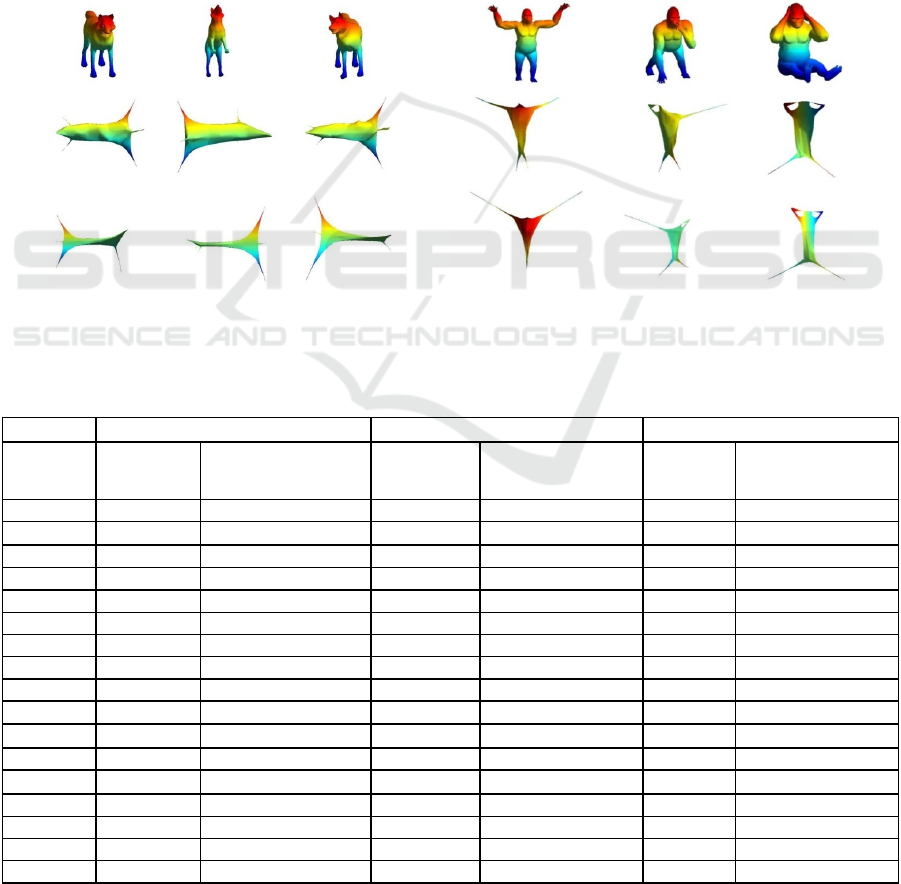
Figure 1: Embedding of wolf and gorilla shapes into canonical forms. From top to bottom depicts original shape, followed
by canonical form obtained by Spectral MDS, Spectral MDS using biharmonic distance.
Table 1: Shows the data of varying geodesic error threshold D, between the model and probe against the average percentage
of point correspondence.
Animal Shapes Human Shapes All Shapes
Geodesic
error(D)
S-MDS
Pts.(%)
SMDS-Biharmonic
Pts. (%)
S-MDS
Pts. (%)
SMDS-Biharmonic
Pts. (%)
S-MDS
Pts. (%)
SMDS-Biharmonic
Pts. (%)
0 1.1183 1.3707 1.2298 1.2207 1.2413 1.3524
0.0125 4.4088 6.7875 4.452 7.3923 4.8266 7.1525
0.025 12.1579 19.1776 14.7096 20.9908 14.596 19.9216
0.0375 24.7667 40.4431 31.5826 46.061 30.4995 43.1803
0.05 39.3009 63.3398 51.1159 66.3549 48.8439 65.2796
0.0625 49.7646 81.8704 68.9267 81.5946 63.7864 82.0446
0.075 57.1189 91.3908 83.3491 92.5794 75.1602 92.2939
0.0875 62.7122 96.8784 90.7177 97.5841 81.9415 97.3656
0.1 67.3756 98.8709 94.6324 99.2309 86.438 99.0808
0.1125 71.5725 99.6609 98.0789 99.7937 90.1884 99.7827
0.125 76.0111 99.9399 99.2249 99.8841 93.1298 99.9328
0.1375 78.8878 99.9553 99.6353 99.9521 94.6593 99.9761
0.15 81.1456 99.9702 99.7597 100 95.6654 100
0.1625 83.5624 99.9702 99.881 100 96.7655 100
0.175 85.7585 100 99.9575 100 97.6749 100
0.1875 87.1764 100 99.9745 100 98.1592 100
0.2 89.0674 100 99.9915 100 98.8559 100
GRAPP 2019 - 14th International Conference on Computer Graphics Theory and Applications
166
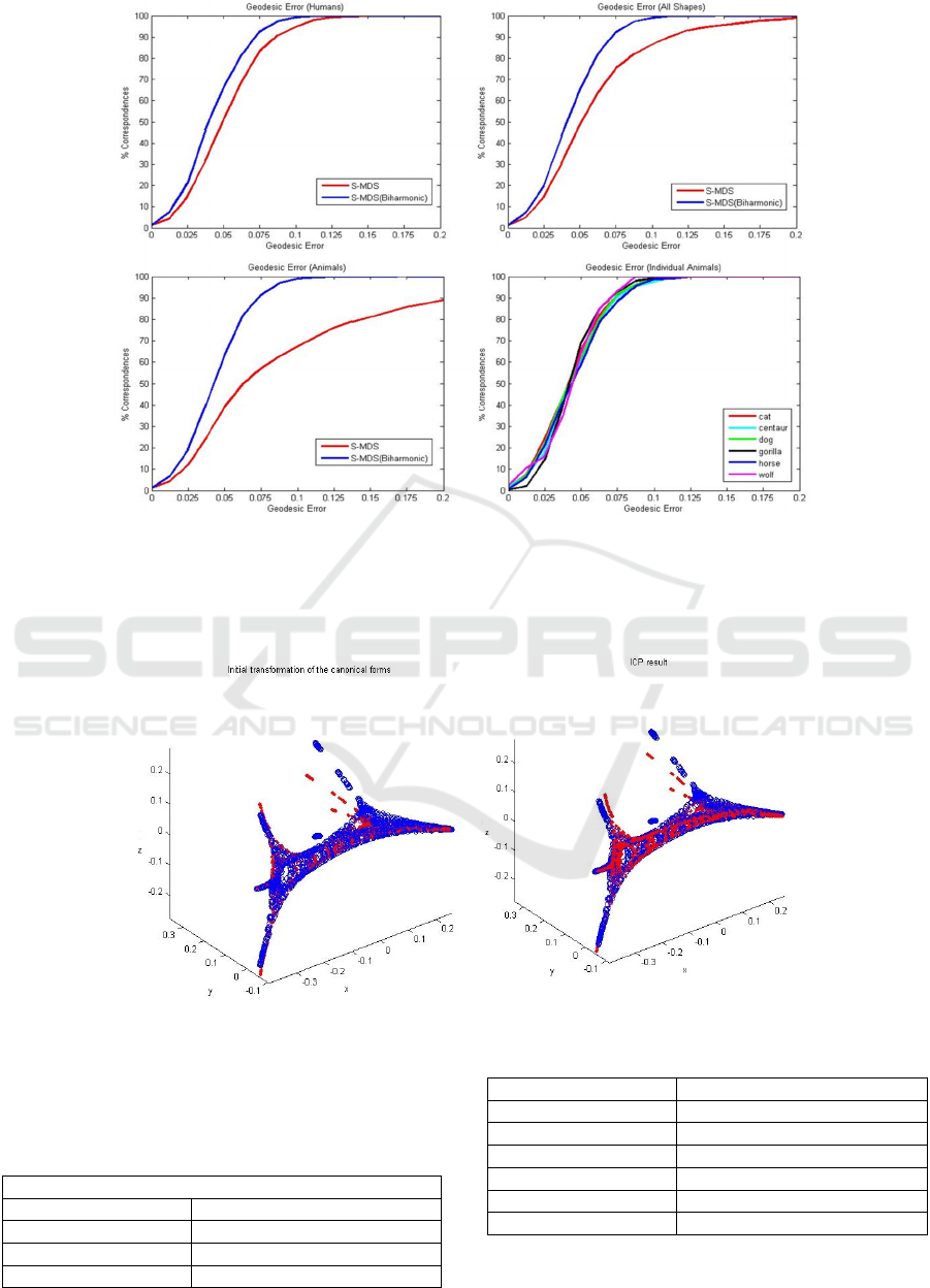
Figure 2: Graphical representation evaluating the geodesic error of correspondence between different categories of shapes.
All graphs show percentage of correspondence between the thresholds of a normalized geodesics error(0-0.2). Top left, top
right and bottom left show comparison of the correspondence between regular S-MDS and S-MDS using biharmonic
distance. Bottom right shows the percentage of correspondence between six different shapes using S-MDS using
biharmonic distance.
Figure 3: An alignment of canonical forms using Iterative Closest Point (ICP) algorithm. From left to right are images of
pre-alignment and post-alignment of two wolf shapes.
Table 2: Comparison of similarity measure function. A
model is compared against ten probes with a threshold
between 0 and 1. The closer the value to 1 the more
similar the model and probe are.
Shape Similarity Measure
Spectral MDS Spectral MDS-Biharmonic
0.9034 0.9117
0.8761 0.8828
0.8720 0.8813
0.8398 0.8505
0.8840 0.8928
0.8565 0.8653
0.7255 0.7282
0.8746 0.8851
0.8987 0.9045
0.8741 0.8821
Spectral Multi-Dimensional Scaling using Biharmonic Distance
167

ACKNOWLEDGEMENTS
The authors would like to thank the reviewers for
their valuable comments. This work is supported by
National Natural Science Foundation of China under
grant No. 61862039, 61462059.
REFERENCES
Vankaick, O., Zhang, H., Hamarneh, G., Cohen-Or, D.,
2011. A survey on shape correspondence, Computer
Graphics Forum, 30(6): 1681-1707.
Sumner, R. W., Popovic, J., 2004. Deformation transfer
for triangle meshes, ACM Transactions on Graphics,
23(3): 399-405.
Kreavoy, V., Sheffer, A., Gotsman, C., 2003.
Matchmaker: constructing constrained texture maps,
ACM Transaction on Graphics, 22(3): 326-333.
Alexa, M., 2002. Recent advances in mesh morphing,
Computer Graphics Forum, 21(2): 173-198.
Jain, A., Zhang, H., 2006. Shape-based retrieval of
articulated 3D models using spectral embeddings, In
Proc. of Geometric Modeling and Processing,
SPRINGER: 295-308.
Bronstein, A. M., Bronstein, M. M., Kimmel, R., 2006.
Generalized multidimensional scaling: a framework
for isometry-invariant partial surface matching, In
Proceedings of the National Academy of Sciences of
the United States of America, 103(5): 1168-1172.
Schwartz, E. L., Shaw, A., Wolfson, E., 1989. A
numerical solution to the generalized mapmaker’s
problem: flattening non convex polyhedral surfaces,
IEEE Transactions on Pattern Analysis and Machine
Intelligence, 11(9): 1005-1008.
Zigelman, G., Kimmel, R., Kiryati, N., 2002. IEEE
Transactions on Visualization and Computer
Graphics, 8(2): 198-207.
Elad, A., Kimmel, R., 2003. On bending invariant
signatures for surfaces, IEEE Transactions on Pattern
Analysis and Machine Intelligence, 25(10): 1285-
1295.
Gromov, M., 1981. Structures metriques pour les varietes
riemanniennes, Textes Mathe´ matiques, 1.
Wolter, F., Reuter, M., Peinecke, N., 2006. Laplace-
Beltrami spectra as ‘shape-DNA’ of surfaces and
solids, Computer-Aided Design, 38(4): 342-366.
Jain, V., Zhang, H., VanKaick, O., 2011. Non-rigid
spectral correspondence of triangle meshes,
International Journal on Shape Modeling, 13(1): 101-
124.
Kim, V., Lipman, Y., Funkhouser, T., 2011. Blended
intrinsic maps, ACM Transactions on Graphics, 30(4):
76-79.
Ovsjanikov, M., Chen, M. B., Solomon, J., Butscher, A.,
Guibas, L., 2012. Functional maps: a flexible
representation of maps between shapes, ACM
Transactions on Graphics, 31(4): 1-11.
Rustamov, R., 2007. Laplace-Beltrami eigenfunctions for
deformation invariant shape representation, In
Symposium on Geometry Processing, SPRINGER:
225-23.
Coifman, R., Lafon, S., 2006. Diffusion maps, Applied
and Computional Harmonic Analysis, 21(1): 5-30.
Sun, J., Ovsjanikov, M., Guibas, L. J., 2009. A concise
and provably informative multi-scale signature based
on heat diffusion, Computer Graphics Forum, 28(5):
1383-1392.
Aubry, M., Schlickewei, U., Cremers, D., 2011. The wave
kernel signature: a quantum mechanical approach to
shape analysis, In Proceedings of the 2011 IEEE
Conference on Computer Vision Workshops, IEEE:
1626-1633.
Aflalo, Y., Kimmel, R., 2013. Spectral multidimensional
scaling, In Proceedings of National Academy of
Sciences, IEEE: 18052-18057.
Lipman, Y., Rustamov, R., Funkhouser, T., 2010.
Biharmonic distance, ACM Transactions on Graphics,
29(3): 27.
Fouss, F., Pirotte, A., Renders, J., Saerens, M., 2007.
Random-walk computation of similarities between
nodes of a graph with application to collaborative
recommendation, IEEE Transactions on Knowledge
and Data Engineering, 19(3): 355-369.
Yen, L., Fouss, F., Deacaestecjer, C., Francq, P., Saerens,
M., 2007. Graph nodes clustering based on the
commute-time kernel, In Proceeding of 11th Pacific-
Asia Conference on Knowledge Discovery and Data
Mining, SPRINGER: 1037-1045.
Grinspun, E., Gingold, Y., Reisman, J., Zorin, D., 2006.
Computing discrete shape operators on general
meshes, Computer Graphics Forum, 25(3): 547–556.
Meyer, M., Desbrun, M., Schrder, P., Barr, A. H., 2003.
Discrete differential-geometry operators for
triangulated 2-manifolds, In Visualization and
Mathematics III, SPRINGER: 35-57.
Bronstein, A. M., Bronstein, M. M., Kimmel, R., 2009.
Numerical geometry of non-rigid shapes, Springer,
New York, 1
st
edition.
Anguelov, D., Srinivasan, P., Pang, H. C., Koller, D.,
Thrun, S., Davis, J., 2004. The correlated
correspondence algorithm for unsupervised
registration of non-rigid surfaces, In Proceeding of
Conference on Neural Information Processing
Systems, MIT PRESS: 33-40.
GRAPP 2019 - 14th International Conference on Computer Graphics Theory and Applications
168
