
Workforce Modelling in Support of Rejuvenation Objectives
Etienne Vincent
Director General Military Personnel Research and Analysis, Department of National Defence,
101 Colonel By Dr, Ottawa, Canada
Keywords: Personnel Modelling, Human Resources Planning, Workforce Analytics, Workforce Demographics,
Rejuvenation, Attrition Rate.
Abstract: This paper presents a method for measuring the effect of staffing policies toward objectives of workforce
rejuvenation. It describes two deterministic models based on the application of rates of personnel flows to
workforce segments. The first model works by solving a system of linear equations describing personnel
flows to obtain the workforce’s age profile at equilibrium. The second model, by iterating through successive
future years, determines the age profile that will result from the set personnel flows. The dynamic model is
necessary to identify shorter term effects of staffing policies.
1 BACKGROUND
This paper describes some elements of a study
conducted for the Canadian Department of National
Defence. The study was requested by the Chief of
Staff for the Assistant Deputy Minister (Science and
Technology). Among this office’s responsibilities is
the management of the Defence Scientific Service
Occupational Classification – a subset of the Federal
Public Service.
At the end of the month of June 2017, there were
616 Defence Scientists. This workforce’s age
distribution is shown in Figure 1.
Figure 1: Workforce age distribution.
The study sponsors believed that this age profile
was less than ideal, as it was thought to contain too
high a proportion of employees that are either
eligible, or close to eligible for retirement. Ideally,
Defence Scientists would acquire expertise over the
course of a long career and pass it on to the next
generation before retirement, through supervision and
mentoring. With relatively few junior employees for
each highly experienced employee approaching
retirement, there was a fear that expertise was not
going to be effectively transferred.
Federal Public Servants are eligible for an
immediate annuity at the age of 65, or at 60 if they
have served at least 30 years. For employees hired
before 2013 the ages are respectively 60 and 55.
Many Defence Scientists retire at the point of first
eligibility, or soon after. For most current employees,
this happens between the ages of 55 and 60.
Otherwise, the amount of the pension still increases
with the number of years of service, up to 35 years,
leading some Public Servants to continue working
past the date of their eligibility for an immediate
annuity. Finally, some chose to continue to work
beyond 35 years of service, despite their annuity no
longer increasing as a proportion of their final salary.
A study of rejuvenation strategies was requested.
The intent of this study was to identify policies that
would result, over time, in a more balanced age
distribution that would allow a better transfer of
expertise from one generation of Defence Scientists
to the next. In particular, the study aimed to predict
the age distribution that could be expected if no
corrective action was taken, and the range of possible
outcomes from potential new staffing policies.
A related study of the Defence Scientist workforce
Vincent, E.
Workforce Modelling in Support of Rejuvenation Objectives.
DOI: 10.5220/0007246700230029
In Proceedings of the 8th International Conference on Operations Research and Enterprise Systems (ICORES 2019), pages 23-29
ISBN: 978-989-758-352-0; ISSN: 2184-4372
Copyright
c
2023 by His Majesty the King in Right of Canada as represented by the Minister of National Defence and SCITEPRESS – Science and Technology Publications, Lda. Under
CC license (CC BY-NC-ND 4.0)
23
was described by Eles and Massel (2008), but that
study focused on career progression, rather than
rejuvenation. Past forecasts for other classifications
of Department of National Defence employees have
often been based on Discrete Event Simulation
(Isbrandt and Zegers, 2006) (Erkelens et al., 2007).
Instead, this paper presents deterministic models
based on the application of rates of personnel flows
to the entire workforce.
2 AGE AT THE TIME OF HIRE
The Defence Scientific Service Classification is
broken down into levels, numbered from 1 to 8. The
level of a Defence Scientist corresponds to his or her
state of career progression, and is tied to a pay scale.
New hires are assigned a level according to an
assessment of their education and prior work
experience. The vast majority of hires are assigned
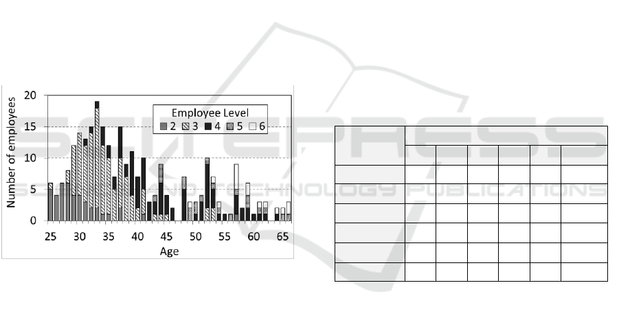
levels between 2 to 6. Figure 2 shows hiring counts,
by level and age, between 1 April 2008 and 30 June
2017.
Figure 2: Age and level of new hires.
New employees are hired on different dates
throughout the year. To facilitate subsequent
analysis, we will be tracking age at the time of hire as
the age of the employee at the end of the fiscal year
in which he or she was hired (31 March). For
example, an employee hired in June, at the age of 50,
and with a birthday in August, will be recorded as
having been hired at the age of 51.
It is seen, in Figure 2, that the level assigned to
new hires tends to increase with their age at the time
of hire. This is because many older hires have
acquired professional and academic experience
warranting a higher level upon becoming Defence
Scientists.
Public Service staffing competitions are always
aimed at specified levels. Prospective employees will
only be hired through competitions that target the
level that is commensurate with their previously
acquired experience. Competitions targeted at lower
classification levels then bring in less experienced
(and thus younger) recruits than competitions
targeting higher levels. Given that age discrimination
is prohibited, younger employees cannot be directly
targeted, but the age profile of the defence scientific
workforce is indirectly a function of the levels
targeted by staffing competitions.
The study described in this paper modelled the
effects of changing the distribution of hiring across
levels on the eventual workforce age profile.
Historically, as shown in Figure 2, approximately
15% of the recruits were hired at level 2, 40% at level
3, 28% at level 4, 8% at level 5 and 7% at level 6
(which does not add up to 100% due to rounding). At
the same time, the mean age at hire was 31 at level 2,
35 at level 3, 46 at level 4, 55 at level 5, and 63 at
level 6. Therefore, any shift of the hiring ratios
toward junior levels would tend to lower the average
hiring age. Table 1 shows six scenarios for different
distributions of hires between the levels. These
scenarios were selected in consultation with the
study’s sponsor.
Table 1: Hiring scenarios to be modelled.
Scenario
A
B
C
D
E
current
level 2
50%
25%
-
20%
20%
15%
level 3
50%
75%
100%
50%
40%
40%
level 4
-
-
-
30%
30%
28%
level 5
-
-
-
-
10%
8%
level 6
-
-
-
-
-
7%
mean age
32.8
33.9
35.1
37.4
39.3
41.2
The scenario denoted as current repeats the
distribution observed in Figure 2. Scenario A, with
50% level 2 and 50% level 3 was thought to be the
most extreme hiring regime that was feasible (new
Ph.D. graduates automatically start at level 3, and
were seen by study sponsors as an unavoidable
recruitment pool). The other scenarios were selected
as plausible regimes that gradually move towards the
age profile of the current scenario. Table 1 also
shows the mean hiring age that would result from
these scenarios, assuming the age distribution of hires
at each level remains unchanged from that observed
in recent years.
ICORES 2019 - 8th International Conference on Operations Research and Enterprise Systems
24

3 ATTRITION
Along with the age at which new employees are hired,
attrition behaviour is the other important determinant
of a workforce’s age profile. We have measured
attrition rates among Defence Scientists as a function
of age. Considering attrition as a function of age has
previously been done in other modelling contexts
(Doumic et al., 2016) (Foran and Straver, 2018).
In order to measure past attrition, we only had
access to annual workforce snapshots broken down
by age. Working from complete records of personnel
flows (hires, departures, occupation transfers, etc.)
would have been preferable, but such data was not
available at the time. Working from annual snapshots
means that we will only model attrition among
employees present at the beginning of the year (thus
excluding attrition among in-year hires), and will
only model counts of net hires (only those that did not
leave during the year when they were hired), instead
of modelling all attrition and hires.
Let
be the number of employees whose
ages are in the range
, at the end of year . A
year earlier,
Defence Scientists
had the potential to be among the
a year
later, but some may have left during year due to
attrition.
By comparing workforce snapshots from
successive years, we can count the number of
employees who were present at the beginning of a
given year, but who departed during the year. Let
be that count during year , among
employees whose ages would have been in the range
at the end of year . Note that this does not
include the departures of new hires who left during
the year when they were hired (those cannot be
obtained from annual snapshots).
To obtain an annual attrition rate, we divide the
count of departures by the headcount at the beginning
of the year. The attrition rate, over year , among
employees who will reach an age in the range
during that year is
(1)
Note that this rate does not fully describe all
attrition, as it only applies to employees who are
present at the beginning of the year. The new hires
over the course of the year may also leave before the
year’s end, but are not factored into Equation (1).
Additional data, beyond the annual workforce
snapshots that we could access, would be necessary
to obtain a rate that also considers in-year attrition
among new hires. The rate given by Equation (1)
underestimates actual attrition, but is for the rate that
will be required by our models.
Attrition rates tend to fluctuate from year to year.
An attrition rate observed one year may not be
representative of the long term trend, and so not
ideally suited for modelling in support of long-term
Human Resources Planning. We thus prefer multi-
year attrition rates, which we compute by
compounding the annual rates obtained from the
annual workforce snapshots using Equation (1). The
attrition rate observed over the multi-year period
starting in year
and ending in year
is obtained
by successively applying the annual rates as
(2)
The resulting multi-year rate can then be
annualized to obtain the annual attrition rate that is
representative of observed trends over the -year
period. We denote the annualized rate
, and
obtain it as
(3)
An alternative would be to use an average, or
weighted average of annual attrition rates, as done by
Okazawa (2007). We prefer to use the annualized
multi-year rate, as it more closely corresponds to a
single rate that would have been in effect over the
whole period. However, we have not investigated
theoretical or empirical reasons for preferring this
rate, over others, in the context of Workforce
Modelling.
We estimated attrition rates using data from April
2008 to March 2017, for age ranges spanning five
years, starting with ages 25 to 29, up to 64, and also
for employees 65 and older. The age ranges were
selected to ensure a sufficient number of person-years
to derive representative rates. There were 133
person-years in the 25 to 29 range, 241 in the 65 and
older range, and substantially more in the other
segments. The resulting rates, based on the period
from 1 April 2008 to 31 March 2017, are shown in
Figure 3.
Attrition is higher among the youngest
employees, who tend to have been recently recruited.
It is then lower for several years. This pattern of
higher attrition in the first years of service is typical
in many workforces, as pointed out by Bartholomew
et al. (1991). Finally, attrition increases greatly after
employees reach the age of 55, corresponding to the
Workforce Modelling in Support of Rejuvenation Objectives
25
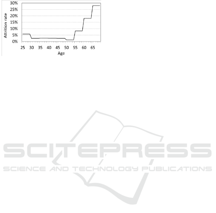
Figure 3: Annual attrition rates.
earliest eligibility for retirement with an immediate
annuity, and in the years after, when all become
similarly eligible. Many also attain the maximum
number of pensionable years (35 for federal Public
Servants).
Among Public Service classifications, Defence
Scientists have comparatively low attrition. This is
likely due to the fact that the specialised expertise of
many Defence Scientists (combining advanced
scientific expertise, and applications to the defence
domain) is not as readily transferable in the wider
labour market. In particular, many other Public
Service classifications are found across government
departments, and so it is common for personnel to
progress in their career by moving from one
department to the next (which counts as attrition,
from an individual department’s perspective).
Defence Scientists are more likely to stay within the
Department of National Defence.
4 EQUILIBRIUM MODEL
Now that we have the age distribution of Defence
Scientists (shown in Figure 1), the hiring age
distribution for selected scenarios (described in Table
1), and the expected attrition rate as a function of age
(shown in Figure 3), we can model the workforce’s
demographic evolution. We start by looking at the
eventual equilibrium that would be reached if hiring
and attrition were to remain unchanged.
At equilibrium, the number of Defence Scientists
remains unchanged from year to year. That is, each
departing employee is replaced by the hiring of
exactly one replacement. In equation terms,
(4)
where is the number of new employees to be hired
each year,
is the number of employees of age
at the beginning of the year, and
is the attrition
rate applicable to employees of age . The sum is
over all ages present in the workforce.
Then, the hired employees are modelled as
following the age distributions associated with the
scenarios in Table 1. Let
be the proportion of
hires whose age will be at the end of the year. In
each scenario,
is the sum over all Defence
Scientist Level, of the products of the proportion of
the hires at each level (from Table 1), with the
proportion of the historical hires at the respective
levels whose age was (which can be observed in
Figure 2).
Each year, employees age by one year, are subject
to the attrition rate for their age band, and are joined
by new hires according to the distribution given by
the
values. Thus, at equilibrium, when the
workforces age profile is steady from year to year,
(5)
Again, Equation (5) does not include in-year
attrition among the new hires. The annual number of
recruits, is net of any in-year attrition, and
was
defined in Section 3 as only applying to employees
present at year-start. Also recall that the age, , is
always the age taken at the end of the year (not at the
time of hire or at the time of attrition).
Equation (5) defines a linear constraint on the age
distribution for each (for this analysis, we have used
ages from 25 to 80). In the resulting system of linear
equations, the values of
and
are
determined from the historical record, and there is an
unknown variable
for each . One more linear
constraint is required to give the system a unique
solution. It is the constraint that the total headcount
be fixed at its current value, which we call (it was
616, on 30 June 2017).
(6)
The system of linear equations defined by
Equations (4), (5) and (6) can now be solved. The
resulting equilibrium age distribution is shown in
Figure 4 for the values of
from the current
scenario.
In figure 4, we see that the equilibrium age
distribution follows a similar profile to the June 2017
age distribution, which is reproduced from Figure 1.
Notice that the equilibrium age distribution is derived
without using the initial state – the close resemblance
between the latest distribution available and the
equilibrium was thus somewhat surprising. The
current age distribution is, thus, close to equilibrium
ICORES 2019 - 8th International Conference on Operations Research and Enterprise Systems
26
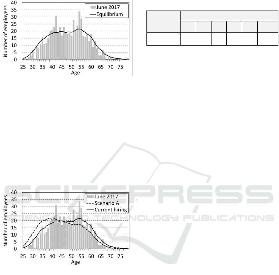
Figure 4: Equilibrium age distributions.
despite successive past periods of boom and bust in
hiring.
To illustrate the impact of modifying the age
distribution of hires on the equilibrium, Figure 5
includes the age profile at equilibrium that results
from hiring as per Scenario A (defined in Table 1).
Scenario A corresponds to the youngest age
distribution that was deemed feasible, and so we can
consider the resulting equilibrium age profile as the
youngest that could realistically be achieved. We see
that this equilibrium distribution is substantially
younger than that obtained for the current scenario
with a peak in the late 30s as opposed to the mid-50s.
Figure 5: Scenario A equilibrium age distributions.
Table 2 shows how each of the hiring scenarios
affects the eventual equilibrium mean age for
Defence Scientists. The mean goes from 48.3 for the
current hiring age profile, to 45.6 under scenario A.
As of 30 June 2017, the time of the latest available
workforce snapshot preceding the study, the mean
age of Defence Scientists in the Department of
National Defence was 48.7. The current scenario
thus leaves the mean age of Defence Scientists
essentially unchanged, while the other scenarios
eventually reduce it. Scenario A achieves the greatest
reduction in mean age, reducing it by 3.1 years.
Table 2: Equilibrium average age for each hiring scenario.
Scenario
A
B
C
D
E
current
Equilibrium
mean age
45.6
46.4
47.1
47.7
48.3
48.8
5 DYNAMIC MODEL
The equilibrium age distributions derived above help
to anticipate the eventual effects of proposed hiring
policies, but do not say what their shorter term impact
will be. Given that public service careers often span
decades, while hiring policies are unlikely to survive
that long, the shorter term effects of a hiring policy
should be of interest. To look at these shorter term
outcomes, a dynamic model is required.
Our dynamic model simply tracks the workforce
composition that results from applying the previously
used attrition rates by age, and replacing departing
personnel with hires, while distributing the ages of
hires according to the distributions from the previous
scenarios. This is defined by Equation (7), which is
like Equation (5), but with added indices to denote
successive years:
(7)
where,
(8)
Equation (8) sets annual hiring to exactly make up
for the year’s attrition. It is identical to Equation (4),
but with an index to denote the year. Figure 6 shows
how the mean age of Defence Scientist would evolve,
over 30 years, under the various hiring scenarios.
Each scenario converges differently toward its
eventual equilibrium. For example, Scenario E starts
with a slight decrease in the mean age over the first
two years, followed by six years of increase, to reach
48.9 years. It then experiences 19 years of decrease,
reaching a low of 48.1 years, before eventually
converging to 48.3 years, as shown in Table 2. The
trajectory of other scenarios reach peaks and troughs
at different points in time on the way to convergence.
After the 30 years shown in Figure 5, it appears that
many scenarios will still fluctuate significantly before
reaching equilibrium.
Figure 7 extends the horizon further into the future
for scenario A, in order to show that the mean age
Workforce Modelling in Support of Rejuvenation Objectives
27
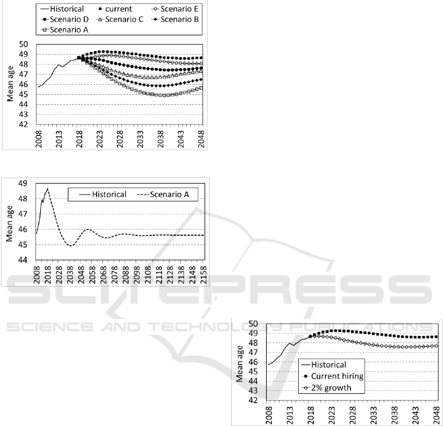
eventually does converge.
Figure 6: Mean age forecast.
Figure 7: Longer term forecast for scenario A.
Figure 7 highlights the fact that although the
dynamic model converges to the value identified by
our equilibrium model, that convergence requires
decades – longer than typical Human Resources
Planning horizons. Therefore, in practice, the
dynamic model that looks at fluctuations over coming
years is necessary for meaningfully comparing hiring
policies.
The oscillation observed on the way to
convergence is something commonly observed in
Workforce Modelling. In this case, the mean age of
the workforce changes with the age distribution
among hires, but it also changes with the number of
hires (hires are generally younger, so more hiring
results in a lowering of the mean age). But lowering
of the mean age, itself, tends to reduce attrition in the
following years, as attrition is highest among the
oldest employees. This lower attrition results in
fewer hires, and thus an ageing workforce. Which
will itself eventually result in increased attrition.
These successive waves of lower attrition / less
hiring / ageing, followed by higher attrition / more
hiring / rejuvenation, continue in a feedback cycle
that gradually tapers off, and eventually converges.
6 WORKFORCE GROWTH
So far, we have studied situations where the
headcount was kept unchanged from year to year.
However, growth or reduction of the workforce, if
they were to occur, would lead to changes in the
workforce’s age profile. To briefly investigate this,
we consider the case of a modest annual growth rate
of 2% in the number of employees.
In order to consider persistent growth or reduction
of the headcount, Equation (8) must be replaced by
(9)
where is the rate of change in the headcount. The
first term of Equation (9) is as Equation (8), and
accounts for the hires that are meant to replace
departing employees. The second term accounts for
the growth or reduction by adding a multiple of the
total headcount. For a negative , corresponding to a
shrinking workforce, Equation (9) only works if the
rate of reduction is lower than attrition. Otherwise,
layoffs are necessary.
Using Equation (9) for a 2% annual growth in
headcount, along with the current scenario for the age
distribution of new hires, we eventually get a
reduction in the mean age of Defence Scientists of
just over one year, as shown in Figure 8.
Figure 8: Mean age forecasts with 2% growth.
If incorporating a growth rate of 2% to the
previously described equilibrium model, we obtain
that the current scenario would then reach a mean age
at equilibrium of 47.7. If combining scenario A (the
one with youngest ages at hire) with the 2% growth
rate, the mean age at equilibrium could fall to 45.0
(compared to the 45.6 without growth in Table 2).
However, the reduction in mean age achieved
through headcount growth is only sustained as long
as the workforce grows. The 2% growth rate used in
our example implies a doubling of the headcount
approximately every 35 years.
ICORES 2019 - 8th International Conference on Operations Research and Enterprise Systems
28

7 CONCLUSIONS
This paper presented two approaches to measuring
the effect of changes in the age distribution of hires
on the age distribution of a workforce. These
methods can inform policy aimed at achieving
workforce rejuvenation. The equilibrium method
leads to an explicit solution for the eventual
equilibrium age distribution, but this equilibrium can
take a very long time to be reached. The dynamic
method then allows us to chart the path taken from the
present toward that equilibrium.
These methods can also be adapted to the analysis
of other workforce demographic characteristics. For
example, they were used by the author to investigate
the impact of hiring policies on the proportion of
women in Defence Scientific Services, in support of
departmental objectives to increase their
representation.
REFERENCES
Bartholomew D.J., Forbes A.F. and McClean S.I., 1991.
Statistical techniques for manpower planning, John
Wiley & Sons. Chichester, United Kingdom, p. 15.
Doumic, M., Perthame, B., Ribes, E., Salort, D. and
Toubiana, N., 2016. Toward an Integrated Workforce
Planning Framework using Structured Equations,
European Journal of Operational Research, 262(1), pp.
217-230. Elsevier. Available at: https://hal.inria.fr/hal-
01343368/document
Eles, P., Massel, P., 2006. DRDC CORA’s OR Scientists:
Analysis of Past Hiring, Career Progression, and
Attrition Trends, and Development of a Model to
Forecast Future Demographics (Centre for Operational
Research and Analysis Technical Memorandum DRDC
CORA TM 2006-31). Defence Research and
Development Canada, Ottawa, ON. Available at:
http://cradpdf.drdc.gc.ca/PDFS/unc71/p529377.pdf
Erkelens, A., Isbrandt, S., Syed, F., 2007. Development of
a Prototype Model for Civilian Occupational Group
Projections, in SummerSim’07, Summer Computer
Simulation Conference, San Diego, CA, USA. Curran
Associates, pp. 1277-1282.
Foran, D., Straver, M., 2017, Forecasting CAF releases and
population: Age-based attrition modelling (Director
General Military Personnel Research and Analysis
Scientific Report DRDC-RDDC-2017-R176). Defence
Research and Development Canada, Ottawa, ON.
Isbrandt, S., Zegers, A., 2006. The Arena Career Modelling
Environment Individual Training and Education
(ACME IT & E) Projection Tool – An Overview (Centre
for Operational Research and Analysis Technical
Report DRDC CORA TR 2006-03). Defence Research
and Development Canada, Ottawa, ON.
Okazawa, S., 2007. Measuring Attrition Rates and
Forecasting Attrition Volume (Centre for Operational
Research and Analysis Technical Memorandum DRDC
CORA TM 2007-02). Defence Research and
Development Canada, Ottawa, ON. Available at:
http://cradpdf.drdc.gc.ca/PDFS/unc66/p527519.pdf
Workforce Modelling in Support of Rejuvenation Objectives
29
