Real-Time Encoding/Decoding for Pairwise Communication Over an

Unreliable Sensor Network

Daniel Graham

, Arnold Yim

, Gang Zhou

and Weizhen Mao

Department of Computer Science, University of Virginia, Charlottesville, VA, U.S.A.

Department of Mathematics and Computer Science, Bridgewater College, Bridgewater, VA, U.S.A.

College of William And Mary, Williamsburg, VA, U.S.A.

Keywords:

Compression Algorithm, Energy Efﬁcient Sensing, Wireless Sensor Networks.

Abstract:

The length of time that a wireless sensor can be deployed is limited by its internal power supply. To increase

the deployment lifetime of these sensors we must ﬁnd ways to conserve power. In this paper, we propose an

algorithm that reduces the amount of energy the transceiver consumes by compressing the bytes that are sent

and received over the network. The algorithm compresses a data stream by exploiting its temporal locality

and is designed to function efﬁciently on an unreliable network in real-time. A stream is compressed by using

fewer bits to represent elements that frequently recur. We evaluate the proposed compression algorithm using

a collection of independently collected traces from the crawdad database. We calculated the compression ratio

for each trace and found that we were able to reduce the number of bytes transmitted by an average of 60%,

resulting in a 30% increase in energy savings.

1 INTRODUCTION

Wireless sensors have been used in a variety of data

collection and monitoring applications. These sensors

are often deployed in locations where they do not have

access to the energy grid and often rely on their in-

ternal energy supply. These locations vary from bat-

tleﬁelds (Keally et al., 2010) and remote geological

locations (Kenney et al., 2009) to deployment within

the human body (Gao et al., 2005). In many cases, re-

placing the batteries in these sensory devices is incon-

venient and costly. Addressing the problem of energy

consumption in wireless sensor nodes will make the

application of sensor nodes more practical.

Real-time compression algorithms have been pro-

posed as a method for improving the energy efﬁciency

of wireless sensors. A real-time compression algo-

rithm reduces the amount of energy the transceiver

consumes by reducing the number of bytes that are

sent over the network.

Though numerous compression algorithms have

been proposed, most of them are not suitable for real-

time use and do not function efﬁciently over an unre-

liable network. The S-LZW (Sadler and Martonosi,

2006) and LEC (Marcelloni and Vecchio, 2008) com-

pression algorithms are currently the state of the art

real-time compression algorithms. Both algorithms

are dictionary compression algorithms, which com-

press data by storing the compressed values and un-

compressed values as key value pairs in a dictionary.

The S-LZW algorithm tailors the original LZW algo-

rithm (Nelson, 1989) to real-time embedded systems.

In particular, the S-LZW algorithm trades the com-

pression ratio of the LZW algorithm for a more efﬁ-

cient use of memory and the ability to tolerate packet

losses. The S-LZW algorithm uses the LZW algo-

rithm to compress the data stream in blocks. This

restricts the size of the dictionary and limits packet

losses to only corrupting sections of the stream. The

LEC algorithm further improves on the compression

ratio of the S-LZW algorithm. Unlike the state of the

art algorithms, the algorithm that we propose in this

paper performs efﬁciently over an unreliable network

without delaying the stream.

The intuition behind the proposed algorithm is

that the sender and receiver will automatically agree

upon a set of codes that they will use to communicate.

Instead of a lengthy message, the sender will trans-

mit a shorter code that conveys the same meaning.

For example, instead of transmitting the 8-bit value

00010100 for the integer 20, the sender instead sends

a 2-bit value 01. The receiver then interprets the value

01 as 00010100. Communicating using a set of codes

reduces the amount of energy the sensor consumes by

Graham, D., Yim, A., Zhou, G. and Mao, W.

Real-Time Encoding/Decoding for Pairwise Communication Over an Unreliable Sensor Network.

DOI: 10.5220/0007247000690076

In Proceedings of the 8th International Conference on Sensor Networks (SENSORNETS 2019), pages 69-76

ISBN: 978-989-758-355-1

reducing the number of bytes a node’s transceiver has

to send and receive.

We evaluate the proposed algorithm by using it

to compress traces from Columbia University’s En-

HANTS dataset (Gorlatova et al., 2011a). The En-

HANTS dataset contains irradiance (light) readings

collected using TAOS TSL230rd photometric sensors.

The photometric sensors were placed in different lo-

cations and readings were collected at 30 second in-

tervals for 392 days. We compress the traces using

both the proposed algorithm and the LZW algorithm.

We compare the performance of the algorithms us-

ing four metrics: compression ratio, energy efﬁciency,

memory usage, and the delay the algorithm induces

on each packet. We evaluate the energy efﬁciency of

the algorithms using the energy model for the cc2420

transceiver proposed by D Schmidt et.al (Schmidt

et al., 2007).

The proposed algorithm improves on the state

of the art algorithms by efﬁciently tolerating packet

losses and reducing the delay induced on the data

stream. This paper makes three contributions:

• Presents a distributed real-time compression algo-

rithm that compresses a data stream by exploiting

its temporal locality.

• Extends the algorithm to ensure that it operates on

an unreliable network.

• Evaluates the compression performance and en-

ergy efﬁciency of the algorithm using traces col-

lected by independent researchers.

The remainder of the paper is structured as fol-

lows: Section 2 presents the compression and decom-

pression algorithm. Section 3 discusses the algorithm

and proves its correctness. Section 4 evaluates the al-

gorithm. Section 5 surveys the related work. Section

6 concludes the paper.

2 THE TEMPORAL

COMPRESSION ALGORITHM

(TCA)

Designing a real-time lossless compression algorithm

presents three unique challenges. The ﬁrst challenge

is designing an algorithm that is able to compress data

without having access to the entire data stream.

The second challenge is ensuring that the algo-

rithm works on an unreliable network. This means

that the algorithm should still be able to decompress

subsequent elements if an element in the series is lost.

The third challenge is maintaining the consistency

of the distributed encoding table on the sender and re-

ceiver. An encoding table is the data structure that

is used to compress and decompress the stream. In

a non real-time application the encoding table is con-

structed and sent along with the compressed data so

that the compressed data can be decompressed later.

However, in a real-time scenario it is not feasible to

wait to send a decompression table since the receiver

must decompress the values in real-time. This means

that both the sender and receiver must either agree on

the decoding table beforehand or independently gen-

erate the same decoding table in real-time.

Encoding tables provide a mapping from the origi-

nal bytes to their compressed representations. For ex-

ample, an encoding table would map the original bits

1111 to the encoding 01. Table 1 shows an example

of an encoding table with 3 entries. An encoding table

Table 1: Example of an encoding table.

00 1001

01 1111

10 1000

can also be used to map a series of uncompressed val-

ues to a series of compressed values. For example the

values {1111, 1001, 1000, 1111} are mapped to the

values {01, 00, 10, 01}. The same encoding table can

also be used to decompress a series of values since

it is a one-to-one mapping. For example, the series

{01, 00, 10,01} can be decompressed using the same

encoding table, thus resulting in the reverse mapping:

{01, 00, 10,01} → {1111, 1001, 1000, 1111}.

Formally, we can think of an encoding table as a

one-to-one function f that maps the original value v to

its compressed form c. Written more brieﬂy, f : v 7→ c.

Values are encoded by using the function f to ﬁnd the

corresponding encoding.

Values are decoded using the inverse of f . The

inverse function f

−1

maps the compressed value c to

its original value v. The decoding function can be

written more brieﬂy as: f

−1

: c 7→ v.

Encoding tables are usually implemented using

associative arrays or hashmaps. The keys of the

hashmap represent the compressed values and the en-

tries represent the original values. We can think of

each entry in the hashmap as an evaluation of the f

−1

for a speciﬁc compressed value v.

Encoding tables are normally used by a class of

compression algorithms called dictionary encoders.

Dictionary encoding algorithms compress data by

reading all the data and constructing an encoding ta-

ble which is then packaged along with the compressed

data, so that it can be decompressed later.

Creating an encoding table for all the data is not

feasible in a real-time scenario, since the algorithm

will not have access to all the data beforehand. This

means that the algorithm on the sender must dynam-

SENSORNETS 2019 - 8th International Conference on Sensor Networks

ically create the encoding table and communicate it

without affecting the real-time constraints of the ap-

plication.

Algorithms 1 and 2 show how the sender and re-

ceiver dynamically create the encoding table without

any communication overhead. The algorithms dy-

namically create an encoding table by caching the last

N values. A value’s encoding corresponds to its index

in the encoding table. If a value reoccurs, the algo-

rithm compresses it by reporting its index in the en-

coding table. If a value is added to an encoding table

for the ﬁrst time the algorithm reports the value in-

stead of the index. Reporting the value instead of the

index allows the receiver to update its encoding table

so that it is consistent with the sender.

During the remainder of this section, we discuss a

detailed example. We use this example to explain how

algorithms I and II are used to establish the distributed

encoding tables dynamically.

Algorithm 1: Algorithm For Compressing

Packets.

Input: Packet To Encode (PTE) ,

N-bitCounter, Encoding Table

Output: Encoded Packet (EP)

if PTE is an entry in the Encoding Table then

EP←Index of the [Entry] return EP

else

Increment N-bitCounter

Encoding← N-bitCounter Add Entry

[PTE] at Index [Encoding] return PTE

end

Algorithm 2: Algorithm For Decompressing

Packets.

Input: Packet To Decode (PTD) ,

N-bitCounter, Encoding Table

Output: Decoded Packet (DP)

if length(PTD)≤ log

(N) then

DP←Entry in Encoding Table at Index

PTD return DP

else

Increment N-bitCounter

Encoding← N-bitCounter Add Entry

[PTD] at Index [Encoding] return PTD

end

Figure 1 shows an example of how the datastream

{1111, 1010, 1111,0000} is compressed and decom-

pressed in real-time. As the ﬁrst value 1111 arrives,

it is inserted at the ﬁrst index in the encoding table.

In this example, we consider an encoding table that

holds a maximum of two encoding pairs. Each value

is encoded using the index of the value in the table.

Ϭ ϭϭϭϭ

ϭ ϭϬϭϬ

Ϭ ϭϭϭϭ

ϭ ϭϬϭϬ

Ϭ ϭϭϭϭ

ϭ ϭϬϭϬ

Ϭ ϭϭϭϭ

ϭ ϭϬϭϬ

Ϭ ϬϬϬϬ

ϭ ϭϬϭϬ

Ϭ ϬϬϬϬ

ϭ ϭϬϭϬ

ϭϭϭϭ

ϭϬϭϬ

ϭϭϭϭ

ϭϬϭϬ

ϭϭϭϭ

ϬϬϬϬ

Figure 1: The diagram above shows an example of how the

algorithm compresses and decompresses a stream of infor-

mation in real-time.

Since the value 1111 is the ﬁrst in the series it is in-

serted at the ﬁrst index in the encoding table: 0. This

is because there are two positions in the table and each

position can be addressed using a single bit. The value

0 corresponds to the ﬁrst position while value 1 cor-

responds to the second position in the table. We use

the 1-bit counter to track the next available position in

the decoding table. In this example the encoding table

is restricted to a maximum of two encoding pairs so

we use a 1-bit counter to represent the index values

{0, 1}.

Once the value 1111 is placed into position 0 the

following encoding pair {1111} → {0} is created.

The sender then sends the value 1111 to the receiver,

so that the receiver can establish the same encoding

pair for the value 1111. Upon receipt of the update

value 1111 the receiver inserts the value at the ﬁrst in-

dex of its decoding table, thus creating the following

encoding pair {0} → {1111}. Now that the decoding

table on the receiver has been synced with the encod-

ing table on the sender, the next time the sender en-

counters the value 1111 it can simply send the com-

pressed value 0 and the receiver will be able to de-

compress the value and interpret it as the value 1111.

Both the sender and receiver maintain a 1-bit

counter. Upon encountering a new value both the

sender and receiver increment the 1-bit counter. If

both counters on the sender and receiver start with

the same index value, every entry will be assigned the

same encoding value on the sender and receiver since

both counters are incremented in sync.

The compression and decompression algorithms

follow the same procedure for the next value 1010.

Since the value is not contained in the encoding table

it will be added to the encoding table. So both al-

gorithms increment their 1-bit counters and insert the

value into the encoding table at position 1.

However, the third packet is treated differently be-

cause the packet is already contained in the encoding

table of the sender. This implies that the encoding

scheme has already been established for this packet.

Therefore, the sender sends the encoded value 0 in-

stead of the value of 1111. The Receiver checks the

Real-Time Encoding/Decoding for Pairwise Communication Over an Unreliable Sensor Network

length of the value and determines that it corresponds

to an encoding value. It then looks up in the encod-

ing table and returns the value at position 0 which is

1111.

Limiting the size of the encoding table helps

decrease the lookup time so that the compression

and decompression processes meet the real-time con-

straints of the application. An N-bit counter only al-

lows for 2

possible encoding keys. The 1-bit counter

in this example only allows for two encoding keys.

When the fourth value (0000) arrives, all the en-

tries in the encoding table have been ﬁlled. Therefore

one of the entries must be overridden, since the en-

coding table can only hold two unique entries. The

ﬁrst value is overwritten, since the N-bit counter is

cyclic, so the fourth packet is placed at the ﬁrst index.

This does not affect the consistency of the encoding

tables, since the counters are cyclic, both the sender

and receiver override the same value in the encoding

table.

3 DISCUSSION OF TEMPORAL

COMPRESSION ALGORITHM

3.1 Proof of Correctness

Let S be a stream of packets {p

, p

....p

}. Let f

)

denote the compression function implemented using

a hashmap of size x. Recall that this hashmap rep-

resents the encoding table that was described earlier

in this section. We formally deﬁne the compression

function below in equation 1.

) =



if H

) =

) otherwise

(1)

The function H

) denotes the hash function that

is applied to the packets. We denote the length of a

packet as |p

|. We detect compressed packets by ex-

amining their length |p

| ≤ log

(x). The decompres-

sion function is formally denoted below.

) =



if |p

| > log

(x)

−1

) if |p

| ≤ log

(x)

(2)

Theorem 1 (Dictionary Consistency). The dictionary

on the sender s remains consistent with the dictionary

on the receiver r for any arbitrary data stream of or-

dered packets.

Proof. To prove the correctness of the algorithm we

must show that the following invariant holds.

Invariant:

( f

)) = p

(3)

Maintenance of Invariant: We must prove that

the invariant holds in two cases. The ﬁrst case is when

the packet is not in the hash table, while the second

case is when the packet is in the hash table.

In the ﬁrst case the packet has not been com-

pressed and |p

| ≥ log

(x) and therefore the decom-

pression function correctly returns the value. The in-

variant holds in this ﬁrst case.

In the second case, equation 4 must be true for the

invariant to hold.

−1

)) = p

(4)

Equation 4 is true by construction, since every key

value pair that is inserted into the hash table H

)

is also inserted as an inverse key value pair in the

−1

) in which the value is treated as the key and

the key is treated as the value.

Termination: The algorithm will terminate be-

cause the data stream is of ﬁnite length and the al-

gorithm only operates on each packet once. The al-

gorithm has a time complexity that is linear with the

number of packets.

3.2 Dealing with Packet Losses

In this section we demonstrate how the proposed al-

gorithm deals with packet losses. To aid our explana-

tion, we introduce three categories of packets: update

packets, compressed packets and locking/unlocking

packets. Update packets cause new key value pairs

to be inserted into the encoding table. compressed

packets contain the encoded values. Locking packets

are used to lock the encoding table, while unlocking

packets are used to unlock the encoding table. Lock-

ing the encoding table prevents new packets from be-

ing added to the encoding table.

The loss of a compressed packet is naturally tol-

erated by the algorithm, since compressed packets do

not affect the consistency of the encoding table. How-

ever, if an update packet is lost the encoding table on

the sender will become inconsistent with the encod-

ing table on the receiver. There are two methods for

ensuring the consistency of the encoding tables. The

ﬁrst method uses acknowledgments to guarantee the

delivery of update packets, while the second method

prevents a lost update packet from updating the en-

coding tables by locking the encoding tables. Each

method has trade-offs. The ﬁrst method is suited for

periods of high temporal locality, while the second

method is suited for periods of low temporal locality.

SENSORNETS 2019 - 8th International Conference on Sensor Networks

^ Z

Ă Đ Ŭ

^ Z

Ă Đ Ŭ

Z Ğ Đ Ğ ŝǀ Ğ Ě

> Ž Ɛƚ

ZĞ ũĞĐƚW ͛

 Đ Đ Ğ Ɖ ƚ W ͛

Figure 2: A Karnaugh map showing a visual proof that

the algorithm guarantees delivery of all update and control

packets under different loss conditions. P

represents the

duplicate packet while X represents a lost packet.

The proposed algorithm accommodates data streams

with sections of both high and low temporal locality

by using both methods. The ﬁrst method is discussed

in subsection 3.3 And the second method is discussed

in subsection 3.4

3.3 Using Acknowledgments for Update

Packets

The sender and receiver use acknowledgments to

guarantee the delivery of update packets, locking

packets, and unlocking packets. The sender starts a

timer and waits for an acknowledgement from the re-

ceiver. Once the sender has sent an update packet

the sender does not update its encoding table or send

another packet until it receives an acknowledgement

from the receiver. If the sender does not receive an ac-

knowledgement within a given time period the sender

resends the packet. The receiver gets a duplicate up-

date packet and resends and acknowledgement. By

using acknowledgments both the sender and receiver

guarantee the consistency of their encoding tables. To

prove that this mechanism works in all scenarios we

use the Karnaugh map shown in ﬁgure 2 to construct

a visual proof.

The ﬁrst cell in the Karnaugh map represents the

condition in which both the packet and the acknowl-

edgment are received. In this case the algorithm func-

tions normally.

The second cell represents the condition under

which the packet is lost but the acknowledgment is

received. This state is not possible since the receiver

will only acknowledge packets that it has received.

The third cell represents the condition under

which an update packet has been received but the ac-

knowledgment has been lost, in which case the sender

retransmits the packet. When the receiver receives the

re-transmitted packet it checks to see if it has already

received the packet by checking the last entry in the

decoding table. If the update packet is already con-

tained in the decoding table, the receiver knows that it

has already received the packet and can conclude that

the acknowledgment was lost. Once the receiver has

concluded that the acknowledgement has been lost it

retransmits the acknowledgement to notify the sender

that it has received the packet.

It may seem that this recovery strategy would

fail if the stream contains two consecutive and iden-

tical update packets since this strategy would drop

the second packet. However, update packets can-

not be duplicated in a sequence. By deﬁnition, if

the packet following an update packet is identical

to the update packet it will be encoded using the

update packet’s index, thus making it a compressed

packet. Consider the following example data stream:

{0001, 0010, 0010}. The second packet 0010 is a

compressed packet since the ﬁrst packet would have

already been stored in the update table. So, instead of

sending the value 0010, the algorithm would transmit

the index, which is a compressed packet.

The fourth cell represents the condition under

which the update packet is lost. If an update packet

is lost, the algorithm will follow the same procedure

described above to ensure that the encoding tables

are kept consistent. It should be noted that using ac-

knowledgements would result in a slight delay since

sender and receiver would wait until the acknowledg-

ment is received.

The algorithm tolerates out-of-order arrivals for

compressed packets but does not tolerate out-of-order

arrivals for update packets. However, this is not a

problem because the algorithm ensures the in-order

arrival of all update packets by buffering the stream

until it has received an acknowledgment.

3.4 Locking the Encoding Table

Acknowledging packets introduces additional delay,

since the sender must wait for an acknowledgement

before allowing the stream to progress. Such delays

may outweigh the beneﬁts of the compression algo-

rithm. This is tolerable, if update packets are rare then

acknowledgments are rarely sent. However, if update

packets are common then acknowledgments have to

be sent frequently. Frequent update packets imply low

temporal locality and the beneﬁts of the compression

may not be worth the delay. To mitigate this we pro-

pose locking the encoding table. Locking the table

stops any additional packets from being added to the

encoding table; thus removing the need for acknowl-

edgments.

To ensure that the algorithm functions efﬁciently

we lock the table during periods of low temporal lo-

Real-Time Encoding/Decoding for Pairwise Communication Over an Unreliable Sensor Network

cality and unlock the table during periods of high tem-

poral locality. We propose using the number of unique

packets within a given time period as a measure of

temporal locality and propose locking the table when

the rate of unique packets rises above a ﬁxed thresh-

old and unlocking the encoding table when the rate

of unique packets falls below a set threshold. This

threshold is determined empirically.

4 EVALUATION

We have evaluated the proposed Temporal Compres-

sion Algorithm using four metrics: 1) the compres-

sion ratio, 2) the energy used by the transceiver, 3)

the number of bytes required for compression. We

use these metrics to compare the temporal compres-

sion algorithm to the state of the art LZW algorithm.

The the temporal compression algorithm reduces the

amount of energy used by the transceiver by 30%

when compared with the uncompressed data stream.

The temporal compression algorithm does not delay

any packets, while the LZW algorithm delays an av-

erage of 80% of the packets.

We evaluate the performance of our algorithm by

examining four traces of irradiance readings obtained

from Columbia University’s EnHANTs dataset (Gor-

latova et al., 2011b). The readings were collected

at 30 second intervals using TAOS TSL230rd photo-

metric sensors installed on LabJack U3 DAQ devices.

Each trace was collected from a sensor placed in a

different location. The ﬁrst trace (Setup A) was col-

lected from a sensor placed on the windowsill of a

south-facing window on the 6

ﬂoor of a building.

The second trace (Setup B) was collected from a sen-

sor placed on top of a bookshelf; this sensor only re-

ceived light for a short portion of the day. The third

trace (Setup C) was collected using a sensor placed on

the windowsill of a north-facing window in a confer-

ence room where the shades were frequently adjusted.

The forth trace was collected by holding a sensor and

walking around time square in New York City.

4.1 Compression Performance

We evaluate the compression performance of an algo-

rithm by calculating its compression ratio. The com-

pression ratio is calculated by dividing the size of the

compressed data by the size of the original data. A

compression ratio of 0.5 means that the compressed

data is half the size of the original data. We calculate

the compression ratio of the TCA algorithm and com-

pare it to the compression ratio of the LZW algorithm.

0 0.5 1 1.5 2 2.5 3

x 10

100

150

Time(Seconds)

Irradiance(/muJ)

(a) Irradiance Readings

Frozen/UnFrozen

Time(Seconds) x 10

0.3 0.6 0.9 1.2 1.5 1.8 2.1 2.4 2.7 3.0

(b) State of Encoding Table

0 0.5 1 1.5 2 2.5 3

x 10

Time(Seconds)

Total Bytes Transfered

TCA 2 bits

TCA 7 bits

uncompressed 8 bits

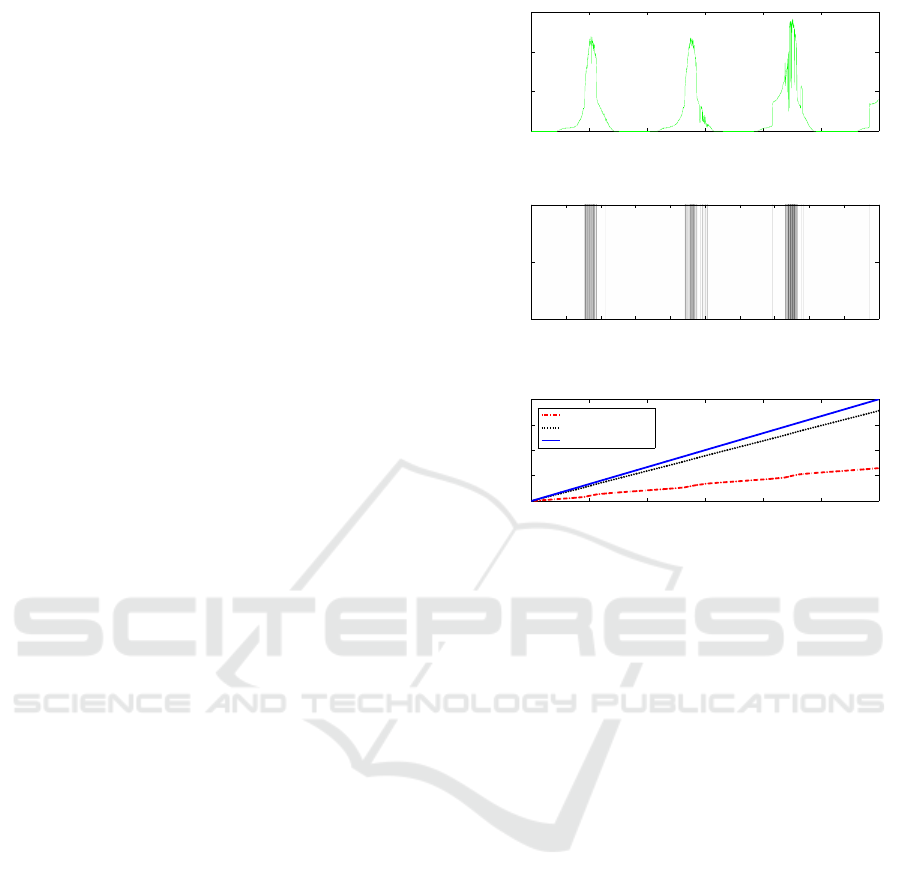
Figure 3: Figure (a) shows the irradiance reading vs time.

Figure (b) is a color map. This color map shows the state

of the encoding table. Dark regions represent a locked state

while light regions represent an unlocked state. Figure (c)

shows the total number of bytes transmitted.

Figure 3(a) shows 10,000 irradiance readings col-

lected over a period of 83.333 hours (3.5 days). These

readings were taken from the trace associated with

setup A. Notice the periodicity between the low ir-

radiance readings and high irradiance readings.

Figure 3(b) shows a colormap. The x-axis shows

the time, while the color of the map represents the

state of the encoding table. Dark regions indicate that

the encoding table is in a locked state, while light

regions indicate that the encoding table is in an un-

locked state. We ran the TCA algorithm using a table

size of four and a threshold of four update packets

every two minutes. As expected dark regions on the

map correspond to sections of low temporal locality

while light regions of the map correspond to sections

of high temporal locality. Therefore we conclude that

using a threshold to identify sections of high and low

temporal locality is an effective strategy for determin-

ing when to lock and unlock the encoding table.

Figure 3(c) shows the total number of bytes vs.

time. The solid blue line represents the total num-

ber of bytes that would be transferred if the stream

was uncompressed (8 bits). The dotted black line

represents the total number of bytes that would be

transferred if the data was compressed using the 7-

SENSORNETS 2019 - 8th International Conference on Sensor Networks

Table 2: (NC) No Compression, (TCA) Temporal Compression Algorithm, (LZW) Lempel Ziv Welch Algorithm.

Trace Algorithm Compression Ratio Memory (bytes) Energy Range (J)

Setup A EnHANTs TCA 0.3233 4 0.0144 → 0.0246

LZW 0.1605 930 0.0030 → 0.0055

Setup B EnHANTs TCA 0.2626 4 0.0139 → 0.0236

LZW 0.0546 401 0.0009 → 0.0018

Setup C EnHANTs TCA 0.2978 4 0.0142 → 0.0242

LZW 0.0791 523 0.0015 → 0.0026

Mobile Trace EnHANTs TCA 0.7261 4 0.0064 → 0.0113

LZW 0.5121 1050 0.0034 → 0.0062

bit encoding temporal compression algorithm. The

dashed red line represents the total number of bytes

that would be transferred if the data was compressed

using the 2-bit encoding temporal compression algo-

rithm.

Figure 3(c) shows how increasing the number of

encoding bits affects the compression ratio. Using

a 2-bit encoding scheme achieves a better compres-

sion ratio than using a 7-bit encoding scheme, because

the 2-bit encoding scheme allows for smaller encoded

packets, which makes up for its inability to capture the

diversity in the stream since it only encodes 4 values

). Though a 7-bit encoding scheme encodes up to

128 values, the compressed packets are 7-bits, 5 bits

larger than the encoded packets used by the 2-bit en-

coding scheme. Since the sections of the data stream

that exhibit high temporal locality contain less than

4 unique values; the 2-bit encoding scheme is better

suited for this trace.

We found that the temporal compression algo-

rithm is able to achieve an average compression ra-

tio of 0.398. This means that the temporal compres-

sion algorithm allows the transceiver to transmit an

average of 60% fewer bytes than the uncompressed

stream.

4.2 Energy Efﬁciency

The energy model for the CC2420 transceiver pro-

posed in (Schmidt et al., 2007) is used to evaluate

the energy efﬁciency of the algorithms. The CC2420

transceiver is commonly found in sensor nodes like

micaz (Polastre et al., 2005).

It is not energy efﬁcient to send a payload that is

only 8 bits long, since 18 bytes of additional informa-

tion must be transmitted along with it. Several sensing

applications solve this problem by packaging multiple

packets into the 28 byte payload. The receiver recov-

ers the packets by parsing the payload. When simulat-

ing the energy consumption of the LZW and tempo-

ral compression algorithm we place multiple packets

in the payload of each data frame. Each data frame

Figure 4: 802.15.4 frame layout.

is packed with 24 packets. Each packet may be an

update packet or a sparse packet. A 24 bit boolean ar-

ray is used to indicate the index of sparse packets and

update packets. A boolean value of 1 means that the

packet is an update packet while a boolean value of 0

means that it is a sparse packet. The boolean array is

stored at the beginning of the frame’s payload. The

receiver uses the boolean array to parse the frame’s

payload.

Figure 4 shows an example of a data frame. The

payload in this example is approximately 4 bytes long

and contains 2 update packets and 2 sparse packets.

Typical payloads will contain 24 packets, however for

the purpose of this example we only show 4 packets.

Since the payload only contains 4 packets, 4 bits of

payload are reserved for the boolean array {1, 0,1, 0}.

The receiver uses this boolean array to parse the pay-

load. A boolean value of 1 means that the receiver

should read the next 8 bits as the value for the up-

date packet, while a value of 0 means that the receiver

should read the next 2 bits as the value for the sparse

packet. In our experiments the payload was ﬁlled with

24 packets. This results in a boolean array that is only

3 bytes long.

5 RELATED WORK

Dictionary coding algorithms have been proposed as

an alternative to tree based encoding algorithms. Dic-

tionary coding algorithms encode values by storing

the compressed value and the original value as key

Real-Time Encoding/Decoding for Pairwise Communication Over an Unreliable Sensor Network

value pairs in a dictionary. This results in fast encod-

ing and decoding times but does not address the space

constraints of embedded devices, as the dictionaries

can become very large.

The LZ77 algorithm encodes data using a dictio-

nary and sliding window (Ziv and Lempel, 1977) .

The algorithm works by sliding an expanding window

across the bytes stream. If the bytes in the window are

in the dictionary the algorithm reports the index of the

bytes. If the bytes in the window are not in the dic-

tionary the algorithm adds the bytes to the dictionary.

However, the LZ77 algorithm does not meet real-time

constraints as the entire data stream is needed in ad-

vance to construct the dictionary.

The LZW algorithm (Nelson, 1989) attempts to

address some of the real-time constraints of the LZ77

algorithm. The LZW algorithm is also a dictionary

coding algorithm and is a modiﬁcation of LZ78 (Ziv

and Lempel, 1978), which is based on the LZ77 com-

pression algorithm. The LZW algorithm starts by ini-

tializing the dictionaries on the sender and receiver

with 256 entries. As the sender gets values it encodes

the values using the dictionary. If the sender gets a

value that is not in the dictionary it adds the value to

the dictionary and sends the value to the receiver so

that it can also add the value to its dictionary. This

is how the algorithm ensures that both the dictionar-

ies on the sender and the receiver are consistent while

still meeting the real-time constraints. However, this

algorithm fails if a single packet is lost. The loss of a

single packet corrupts the dictionaries. The algorithm

does not impose a size constraint on the dictionaries.

This means that the dictionaries can grow to be very

large. It is difﬁcult to store large dictionaries on sen-

sor devices with limited memory.

The S-LZW (Sadler and Martonosi, 2006) algo-

rithm was introduced to address the memory con-

straints and packet loss constraints of the LZW algo-

rithm. The S-LZW algorithm restricts the dictionary

to 512 entries and divides the data stream into inde-

pendent blocks. A new dictionary is created for each

block. If the dictionary is ﬁlled, it is frozen, and no

new entries are added.

6 CONCLUSION

In this paper we present a real-time compression and

decompression algorithm for unreliable networks.

The algorithm compresses a data stream by exploiting

the stream’s temporal locality. Fewer bits are used to

represent elements that frequently recur in a tempo-

ral sequence. The sender and receiver automatically

agree upon the bits that will be used to encode the el-

ements. These bits are then stored in encoding tables

which are used to compress and decompress the data

in real-time.

REFERENCES

Gao, T., Greenspan, D., Welsh, M., Juang, R., and Alm,

A. (2005). Vital signs monitoring and patient tracking

over a wireless network. In Engineering in Medicine

and Biology Society, 2005. IEEE-EMBS 2005. 27th

Annual International Conference of the, pages 102–

105.

Gorlatova, M., Wallwater, A., and Zussman, G. (2011a).

Networking low-power energy harvesting devices:

Measurements and algorithms. In INFOCOM, 2011

Proceedings IEEE, pages 1602–1610. IEEE.

Gorlatova, M., Zapas, M., Xu, E., Bahlke, M., Kymissis,

I. J., and Zussman, G. (2011b). CRAWDAD data set

columbia/enhants (v. 2011-04-07). Downloaded from

http://crawdad.cs.dartmouth.edu/columbia/enhants.

Keally, M., Zhou, G., and Xing, G. (2010). Watchdog: Con-

ﬁdent event detection in heterogeneous sensor net-

works. In Real-Time and Embedded Technology and

Applications Symposium (RTAS), 2010 16th IEEE,

pages 279–288.

Kenney, J., Poole, D., Willden, G., Abbott, B., Morris, A.,

McGinnis, R., and Ferrill, D. (2009). Precise position-

ing with wireless sensor nodes: Monitoring natural

hazards in all terrains. In Systems, Man and Cybernet-

ics, 2009. SMC 2009. IEEE International Conference

on, pages 722–727.

Marcelloni, F. and Vecchio, M. (2008). A simple algo-

rithm for data compression in wireless sensor net-

works. Communications Letters, IEEE, 12(6):411–

413.

Nelson, M. R. (1989). Lzw data compression. Dr. Dobb’s

Journal, 14(10):29–36.

Polastre, J., Szewczyk, R., and Culler, D. (2005). Telos: en-

abling ultra-low power wireless research. In Informa-

tion Processing in Sensor Networks, 2005. IPSN 2005.

Fourth International Symposium on, pages 364–369.

IEEE.

Sadler, C. M. and Martonosi, M. (2006). Data compres-

sion algorithms for energy-constrained devices in de-

lay tolerant networks. In Proceedings of the 4th inter-

national conference on Embedded networked sensor

systems, pages 265–278. ACM.

Schmidt, D., Krämer, M., Kuhn, T., and Wehn, N. (2007).

Energy modelling in sensor networks. Advances in

Radio Science, 5(12):347–351.

Ziv, J. and Lempel, A. (1977). A universal algorithm for se-

quential data compression. Information Theory, IEEE

Transactions on, 23(3):337–343.

Ziv, J. and Lempel, A. (1978). Compression of individual

sequences via variable-rate coding. Information The-

ory, IEEE Transactions on, 24(5):530–536.

SENSORNETS 2019 - 8th International Conference on Sensor Networks