Planar Motion Bundle Adjustment

Marcus Valtonen

Ornhag

and M

arten Wadenb

ack

Centre for Mathematical Sciences, Lund University, Lund, Sweden

Department of Mathematical Sciences, Chalmers University of Technology and the University of Gothenburg,

Gothenburg, Sweden

Keywords:

Planar Motion, Bundle Adjustment.

Abstract:

In this paper we consider trajectory recovery for two cameras directed towards the ﬂoor, and which are

mounted rigidly on a mobile platform. Previous work for this speciﬁc problem geometry has focused on

locally minimising an algebraic error between inter-image homographies to estimate the relative pose. In or-

der to accurately track the platform globally it is necessary to reﬁne the estimation of the camera poses and

3D locations of the feature points, which is commonly done by utilising bundle adjustment; however, existing

software packages providing such methods do not take the speciﬁc problem geometry into account, and the

result is a physically inconsistent solution. We develop a bundle adjustment algorithm which incorporates the

planar motion constraint, and devise a scheme that utilises the sparse structure of the problem. Experiments

are carried out on real data and the proposed algorithm shows an improvement compared to established generic

methods.

1 INTRODUCTION

Structure from Motion (SfM) is a classic problem in

computer vision, and concerns the simultaneous de-

termination of the scene geometry (the structure) and

the pose of the cameras (the motion) from a number

of images of a scene (Hartley and Zisserman, 2004;

Szeliski, 2011). Modern systems for SfM, such as the

ones famously used to “build Rome” (Agarwal et al.,

2011; Frahm et al., 2010) or the popular Bundler sys-

tem (Snavely et al., 2008), are able to generate im-

pressive reconstructions of increasingly large scenes

from large unordered and unlabelled collections of

images.

Among the key enabling technologies for these

successes in large scale SfM are algorithms for per-

forming Bundle Adjustment (BA), i.e. solving the

SfM problem as a large optimisation problem (Triggs

et al., 1999). In this optimisation problem, a cost

function—often chosen as the sum of squared geo-

metric reprojection errors—is to be minimised with

respect to a set of parameters describing the scene

geometry and the camera poses. Formulating SfM

as a BA problem has a number of beneﬁts when it

comes to the problem modelling, e.g. (a) it can, in a

uniﬁed way, incorporate assumptions concerning the

camera calibration, (b) it allows the use of a suit-

able parametrisation and/or explicit constraints for the

purpose of enforcing a particular motion model, and

meaningful quantity, as opposed to a purely algebraic

error.

Due to its relatively high computational cost, BA

has traditionally been applied mainly in ofﬂine batch

processing systems such as the ones mentioned above.

During the last two decades, however, BA has started

to surface in online SfM systems used for cam-

era based Simultaneous Localisation and Mapping

(SLAM) and Visual Odometry (VO), where it can be

performed at regular intervals e.g. to reduce scale

drift or to improve consistency in general. This devel-

opment has been driven by improvements in the per-

formance of hardware as well as by advances in the al-

gorithms and their implementation, and we anticipate

that more and more application speciﬁc implementa-

tions of BA will move towards real-time systems.

In visual SLAM there is sometimes additional

information available compared to a general SfM

problem, and this can be exploited to improve the

performance of the system. For instance, the im-

ages are acquired in an ordered sequence, and this

avoids expensive “all-vs-all” matching of the images

when searching for correspondences. Another possi-

ble source of valuable information is a suitable mo-

tion model, which can be used e.g. for feature predic-

tion (Davison et al., 2007; Davison, 2003), to exploit

Örnhag, M. and Wadenbäck, M.

Planar Motion Bundle Adjustment.

DOI: 10.5220/0007247700240031

In Proceedings of the 8th International Conference on Pattern Recognition Applications and Methods (ICPRAM 2019), pages 24-31

ISBN: 978-989-758-351-3

non-holonomic constraints (Zienkiewicz and Davi-

son, 2015; Scaramuzza, 2011a; Scaramuzza, 2011b),

or to constrain the camera motion to a plane (Hajj-

diab and Lagani

ere, 2004; Ort

ın and Montiel, 2001;

Wadenb

ack and Heyden, 2014).

In this paper, we will consider BA in the con-

strained planar motion case for a pair of cameras—not

necessarily with overlapping ﬁelds of view—attached

to a mobile platform in such a way that each of the

two cameras are subject to a planar motion model, in

addition to the rigid body motion connecting them.

2 RELATED WORK

An early approach by Ort

ın and Montiel used a pla-

nar motion model to parametrise the essential matrix

between successive views in terms of two translation

parameters and one rotation angle, which allowed the

relative motion to be recovered from two point corre-

spondences using a non-linear solver (Ort

ın and Mon-

tiel, 2001). One limitation of this approach is that

it does not contain any way to determine the length

of the translation between the camera positions. An-

other limitation is that the camera must be mounted

in such a way that the optical axis is horizontal, to a

reasonably high precision, in order to allow the sim-

ple parametrisation employed. A similar approach

was considered for the stereo case in (Chen and Liu,

2006).

In the monocular case, the problems of scale am-

biguity and scale drift are connected to the use of the

fundamental matrix to solve the relative pose prob-

lem. An additional drawback of these methods is

that the fundamental matrix cannot be determined

from co-planar correspondences—see e.g. (Hartley

and Zisserman, 2004) for further discussion of this

degeneracy—which is a considerable issue in indoor

environments where planar structures are common.

These considerations, among others, have led re-

searchers to consider homography based methods in-

stead.

The homography based method by Liang and

Pears used correspondences in the ground plane, to-

gether with a planar motion model (Liang and Pears,

2002). They showed that the rotation angle about the

vertical axis can be found via the eigenvalues of the

homography matrix, regardless of how the camera is

mounted. A similar geometric situation, but allowing

only one tilt angle in the possible camera orientations,

was studied in (Hajjdiab and Lagani

ere, 2004). They

also devised an effective scheme for estimating the

full set of motion parameters.

More recent work by Wadenb

ack and Heyden ex-

tended the homography based methods for planar mo-

tion and co-planar keypoints to the general 5-DoF sit-

uation (Wadenb

ack and Heyden, 2013). Their method

used a decoupling of the underlying 2D rigid body

motion from the camera tilt, which was ﬁrst esti-

mated iteratively. The same general geometric situ-

ation was also considered by Zienkiewicz and Davi-

son, who proposed a dense matching of the images

based on non-linear optimisation for determining the

correct motion parameters (Zienkiewicz and Davison,

2015).

The general 5-DoF situation was extended to a

binocular setup, with possibly non-overlapping ﬁelds

of view, in (Valtonen

Ornhag and Heyden, 2018a;

Valtonen

Ornhag and Heyden, 2018b). The cameras

were assumed to be connected by a rigid body mo-

tion, and it was shown that it is possible to recover the

relative pose between the cameras.

Bundle adjustment is a well-studied problem and

an excellent overview is that of (Triggs et al., 1999),

mentioned in the introduction. Since bundle ad-

justment often involves solving a large system of

equations it is necessary to account for the struc-

ture of the problem, e.g. by exploiting sparsity pat-

terns. One sparse bundle adjustment package avail-

able is SBA (Lourakis and Argyros, 2009), which

utilises the sparsity in the Jacobian matrix by using

Schur complementation in order to speed up the algo-

rithm. The SBA package has been successfully used

in e.g. (Snavely et al., 2008; Agarwal et al., 2011;

Frahm et al., 2010).

Among more recent implementations of sparse

bundle adjustment is Sparse Sparse Bundle Adjust-

ment (sSBA) (Konolige, 2010) and Simple Sparse

Bundle Adjustment (SSBA) (Zach, 2014), which uses

a similar approach as SBA in the sense that the aug-

mented normal equations are solved, but utilises pack-

ages that exploit the sparsity more efﬁciently. To

speed up convergence, and move into the domain

of real-time applications, Parallel Bundle Adjustment

was introduced in (Wu et al., 2011) which supports

GPU acceleration where a preconditioned Conjugate

Gradients (CG) system is solved. Another GPU im-

plementation by H

ansch et al. shows that is is possi-

ble to efﬁciently parallelise the Levenberg-Marquardt

algorithm (LM) (H

ansch et al., 2016). Recent papers

dealing with very large scale SfM problems have suc-

cesfully employed distributed methods, by employing

splitting methods (Eriksson et al., 2016; Zhang et al.,

2017).

Furthermore, choosing the cost function to be the

sum of squared geometric reprojection errors is not

the only viable option—for monocular visual odome-

try photometric bundle adjustment, where the photo-

Planar Motion Bundle Adjustment

metric consistency is maximised, has proven to be a

good competitor (Alismail et al., 2016).

3 THEORY

3.1 Problem Geometry

In this paper we consider a mobile platform with two

cameras directed towards the ﬂoor. The world coor-

dinate system is chosen such that the ground ﬂoor is

positioned at z = 0, whereas the cameras move in the

planes z = a and z = b, respectively. Furthermore,

the ﬁelds of view of the cameras are not assumed to

be overlapping, and both cameras are assumed to be

mounted rigidly onto the platform. Due to this setup,

the cameras are connected by a rigid body motion,

and, without loss of generality, we may assume that

the centre of rotation of the mobile platform is located

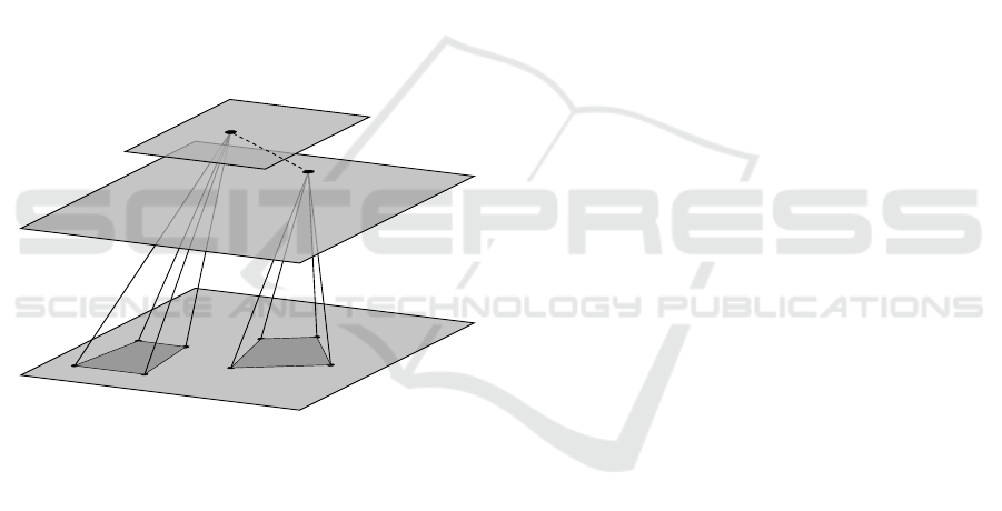
in the ﬁrst camera centre, as is illustrated in Figure 1.

z = 0

z = b

z = a

Figure 1: The problem geometry considered in this paper.

The cameras are assumed to move in the planes z = a and

z = b, the relative orientation between them as well as the

tilt towards the ﬂoor normal is assumed to be constant as the

mobile platform moves freely.

3.2 Camera Parametrisation

A camera parametrisation well suited to the inter-

nally calibrated monocular case of this speciﬁc prob-

lem geometry was derived in Wadenb

ack and Hey-

den (Wadenb

ack and Heyden, 2013), and we adopt

this parametrisation here. The camera matrix associ-

ated with the image taken at position j is thus written

( j)

= R

ψθ

( j)

I | − t

( j)

], (1)

where R

ψθ

is a rotation θ about the y-axis followed

by a rotation of ψ about the x-axis. The movement

of the mobile platform is modelled by a rotation ϕ

( j)

about the z-axis, corresponding to R

( j)

, and a trans-

lation vector t

( j)

. In (Valtonen

Ornhag and Heyden,

2018a) the camera matrices for the second camera are

parametrised as

0( j)

= R

(b)R

( j)

I | −t

( j)

], (2)

where ψ

and θ

are the tilt angles, deﬁned analo-

gously as for the ﬁrst camera, τ

τ is the relative transla-

tion between the camera centres and η is the constant

rotation about the z-axis relative to the ﬁrst camera.

None of the constant parameters are assumed to be

known. The translation matrix T

(b) is deﬁned as

(b) = I

I − τ

τn

/b, where τ

τ =

(τ

, τ

, 0)

, n

n is a ﬂoor

normal and b is the height above the ground ﬂoor. Due

to the global scale ambiguity we may assume a = 1.

4 PREREQUISITES

4.1 Geometric Reprojection Error

Consider the pose of the ﬁrst camera at position j,

given by the camera matrix in (1), and let

( j)

denote

the estimated measurement of the scene point X

homogeneous coordinates, i.e.

( j)

∼ P

( j)

. Let x

( j)

denote the measured image point, and deﬁne the

residual r

i j

as r

i j

= x

( j)

−

( j)

, where

( j)

is the in-

homogeneous representation of

( j)

. Analogously to

the ﬁrst camera, deﬁne the residual r

i j

for the image

of X

in the second camera. Given N stereo camera

locations and M scene points, we seek to minimise

the geometric reprojection error E given by

E(β

β) =

∑

i=1

∑

j=1

i j

+ kr

i j

, (3)

where β

β is the parameter vector consisting of the cam-

era parameters and the scene points.

4.2 The Levenberg-Marquardt

Algorithm

For bundle adjustment it is common to use the

Levenberg-Marquardt algorithm (LM) which solves

the augmented normal equations



J + µI



δ = J

ε, (4)

where J

J is the Jacobian of the cost function and ε

the residual vector. The reader is referred to (Triggs

et al., 1999; Lourakis and Argyros, 2009) for more

details regarding the LM algorithm and its application

ICPRAM 2019 - 8th International Conference on Pattern Recognition Applications and Methods

to bundle adjustment. There are other options to the

LM algorithm, e.g. the dog-leg solver (Lourakis and

Argyros, 2005) and preconditioned CG (Byr

od and

Astr

om, 2010); however, LM is one of the most com-

monly used algorithms today, and is used in modern

systems such as SBA (Lourakis and Argyros, 2009)

and sSBA (Konolige, 2010). Note, however, that SBA

assumes the camera parameters for each camera to be

decoupled, which is not the case for this speciﬁc prob-

lem geometry.

4.3 Initial Solution for Camera Poses

A good initial solution for the camera poses can be

generated using the method described in Wadenb

ack

and Heyden (Wadenb

ack and Heyden, 2014) for the

monocular case. The method takes as input the inter-

image homographies for the path. These can be es-

timated using Direct Linear Transform (DLT) (Hart-

ley and Zisserman, 2004) from point correspondences

established by automatic matching of features, e.g.

SIFT (Lowe, 2004) or SURF (Bay et al., 2006). Re-

gardless of how the homographies are obtained, the

method continues to estimate the overhead tilt R

ψθ

from one or several homographies, and then computes

the translation and orientation about the ﬂoor normal

by QR decomposition of R

ψθ

In order to initialise the stereo parameters the

method proposed in (Valtonen

Ornhag and Heyden,

2018a) can be used. This method relies on the

the estimates from the monocular method described

above, by ﬁrst treating the two trajectories individu-

ally. When the trajectories are known individually,

the relative pose between the two cameras may be ex-

tracted. Both methods beneﬁt from using more than

one homography to estimate the motion of the mobile

platform.

4.4 Triangulation of 3D Points

Linear triangulation of 3D points can be posed as ﬁnd-

ing the null-space of a matrix relating the scene points

and the camera matrices, see e.g. (Hartley and Zisser-

man, 2004); however, this may not result in a physi-

cally meaningful solution in the sense that all points

may not be on the plane z = 0. There is a homog-

raphy between the measured points and the ground

plane; namely, given an image point x

x and the corre-

sponding camera P

P and scene point X

X ∼

(X, Y, 0, 1)

holds that x

x ∼ P

X = H

X. Let P

denote the i:th col-

umn of P

P, then H

H =

]

is the homography we

seek and

X ∼

(X, Y, 1)

contains the unknown scene

point coordinates. It follows that the corresponding

scene point can be extracted from

X ∼ H

−1

Having more than one camera will generally re-

sult in different 3D points; however, all of them will

be on the plane z = 0. We use a simple heuristic to tri-

angulate the points by computing the centre of mass.

This is fast, but suffers from the presence of outliers,

which must be removed prior to triangulation in order

to achieve reasonable performance.

5 PLANAR MOTION BUNDLE

ADJUSTMENT

5.1 Block Structure

Consider the general case of N stereo camera po-

sitions, with M scene points. For convenience, let

γ =

(ψ, θ)

and γ

(ψ

, θ

, τ

, b, η)

denote the un-

known and constant parameters for each camera path

and ξ

(ϕ

( j)

, t

( j)

, t

( j)

)

be the nonconstant parameters

for position j. Then, the Jacobian J

J has the following

block structure:

J =













, (5)

where the derivative blocks are deﬁned as

i j

∂r

i j

∂ξ

, B

i j

∂r

i j

∂

, Γ

i j

∂r

i j

∂γ

i j

∂r

i j

∂ξ

, B

i j

∂r

i j

∂

, Γ

i j

∂r

i j

∂γ

(6)

and where

, Y

)

are the unknown scene coor-

dinates. We write this compactly as

J =



Γ 0

0 A

A B

0 Γ



. (7)

5.2 Utilising the Sparse Structure

As in SBA (Lourakis and Argyros, 2009) and other

similar frameworks, we would like to use Schur com-

plementation; however, it is not directly applicable

Planar Motion Bundle Adjustment

due to the contributions from the constant parame-

ters. Consider, the approximate Hessian J

J in the

compact form

J =



C E



, (8)

where C

C contains the contribution from the constant

parameters, D

D contains the contribution from the non-

constant parameters and the scene points and E

E the

mixed contributions. The matrix D

D may further be

decomposed into

D =



U W



, (9)

with block diagonal matrices U

U = diag(U

,. .. ,U

)

and V

V = diag(V

,. .. ,V

), where

∑

i=1

i j

+ A

i j

∑

j=1

i j

+ B

i j

= A

i j

+ A

i j

(10)

The solution to a system on the form (D

D + µI

I)δ

δ = ε

ε,

where D

D is deﬁned as in (9), is well-known, and is

solved efﬁciently, with minor modiﬁcations, using ex-

isting software packages by utilising Schur comple-

mentation.

The main idea of our method is to incorporate the

constant parameters and consider the decomposition

of (8) as nested Schur complements, which reduces

the problem to the form used in SBA and other well-

established software packages, which in turn can be

efﬁciently solved. To achieve this, consider the aug-

mented normal equations (4) in block form



∗









, (11)

where C

∗

and D

∗

denote the augmented matrices,

with the µ term added on the main diagonals, as in (4).

Applying Schur complementation yields



∗

− E

∗−1

∗







− E

∗−1



(12)

Some remarks are in order. First, note that D

∗−1

appears in (12) twice, and is infeasible to compute

explicitly, which is avoided using the following ob-

servations: introduce the auxiliary variable δ

aux

, such

that

∗

aux

= ε

, (13)

which can be solved with e.g. SBA. In a similar man-

ner D

∗

∆

aux

= E

can be solved by iterating over the

columns of E

. This may at ﬁrst seem like a time

consuming task, however, given that the number of

constant parameters is low—as in the problem geom-

etry considered in this paper—having already solved

for (13), the computation of the Schur complement,

as well as intermediate matrices not depending on the

right hand side, can be stored and reused.

When the auxiliary variables are solved for, it is

possible to compute δ

from



∗

− E

E∆

∆

aux



= ε

− E

Eδ

aux

, (14)

and, ﬁnally, for δ

by back-substitution

∗

= ε

− E

. (15)

Again, note the resemblance of (13) and (15), hence

the computation of the Schur complement and inter-

mediate matrices can be stored and reused.

6 EXPERIMENTS

6.1 Initial Solution

The inter-image homographies were estimated us-

ing the MSAC algorithm (Torr and Zisserman, 2000)

from four point correspondences by extracting SURF

keypoints and applying a KNN algorithm to establish

the matches.

Using all available homographies, the monocular

parameters were recovered by the method proposed

in (Wadenb

ack and Heyden, 2014) and the binocu-

lar parameters using (Valtonen

Ornhag and Heyden,

2018a). The output is given in terms of the relative

pose between the frames, and by aligning the ﬁrst

camera position to the origin the absolute poses for

the remaining cameras can be computed. Knowing

the poses, the scene points were triangulated as dis-

cussed in Section 4.4.

6.2 Choice of Dataset

Due to the lack of a good and established planar mo-

tion evaluation dataset the KITTI Visual Odometry

/ SLAM benchmark (Geiger et al., 2012), was cho-

sen to demonstrate the proposed method. The dataset

contains several sequences and subsequences of pla-

nar or near planar motion, in which a signiﬁcant por-

tion of the images depict the road. There are, how-

ever, sequences containing irregularities in the road

causing the camera to move up and down, which is

not a valid motion according to the planar motion

model. Such sequences were shortened to contain im-

ages where the assumption is a reasonable approxi-

mation. Furthermore, it is known a priori that parts

ICPRAM 2019 - 8th International Conference on Pattern Recognition Applications and Methods

Figure 2: Images from the KITTI Visual Odometry / SLAM benchmark, Sequence 01 (left) and 03 (right). The input images

are cropped (thick border) in order for them to contain a large portion of a near planar surface. This assumption is only valid

in a subset of the sequences, e.g. the highway of Sequence 01 (left). In many cases occlusions, such as the car in Sequence 03

(right), or the non-planar background surface, is not approximated well by the planar motion model. These situations often

occur at road intersections and turns. Image credit: KITTI dataset (Geiger et al., 2012).

of the image is not approximated well by the planar

motion model, e.g. the sky and non-planar structures

often visible on the side of the road. Therefore these

parts are cropped out before estimating the homogra-

phy, see Figure 2.

6.3 Bundle Adjustment Comparison

From the initial trajectory a general 6-DoF model was

used and solved with SBA for both camera trajecto-

ries and compared to the proposed method. For a fair

comparison, no feature points were matched between

the stereo views, as to demonstrate that the overlap-

ping of ﬁelds of view are not necessary to achieve

better performance. The different BA algorithms used

the same settings for termination and control of the

damping parameter µ. The results are shown in Fig-

ure 3.

In all cases the performance of the proposed

method is better or as good as the ones obtained

with the general 6-DoF model and SBA. In the cases

where the initial trajectory is irregular SBA often

converges to a solution where these irregularities are

still present, and thus produces a physically improb-

able solution. This phenomenon is rarely seen in our

method, which converges to a smooth trajectory un-

der fairly general circumstances, regardless of the ini-

tial solution. This holds true even in cases where the

planar motion model is not valid, see e.g. Figure 3(b)

depicting Sequence 03, where the subsequence of the

turn in the road, cf. Figure 2, is non-planar—apart

from the degree of the turn being too sharp, the re-

maining characteristics of the ground truth trajectory

are present, which is not the case for the general 6-

DoF model.

7 CONCLUSION

In this paper we have devised a bundle adjustment

method taking the speciﬁc planar motion problem ge-

ometry into account. An implementation scheme that

utilises the sparse structure of the problem has been

proposed and the method has been tested on sub-

sequences of the KITTI Visual Odometry / SLAM

benchmark and compared to state-of-the-art methods

for sparse bundle adjustment. The results show that

the method performs well and gives a physically rea-

sonable solution, despite some of the model assump-

tions not being fulﬁlled.

ACKNOWLEDGEMENTS

This work has been funded by the Swedish Research

Council through grant no. 2015-05639 ‘Visual SLAM

based on Planar Homographies’.

REFERENCES

Agarwal, S., Furukawa, Y., Snavely, N., Simon, I., Cur-

less, B., Seitz, S. M., and Szeliski, R. (2011). Build-

ing Rome in a Day. Communications of the ACM,

54(10):105–112.

Alismail, H., Browning, B., and Lucey, S. (2016). Photo-

metric Bundle Adjustment for Vision-Based SLAM.

In Asian Conference on Computer Vision (ACCV),

pages 324–341, Taipei, Taiwan.

Bay, H., Tuytelaars, T., and Van Gool, L. (2006). SURF:

Speeded Up Robust Features. In European Confer-

ence on Computer Vision (ECCV), pages 404–417,

Graz, Austria.

Byr

od, M. and

Astr

om, K. (2010). Conjugate gradient bun-

dle adjustment. In European Conference on Computer

Vision (ECCV), pages 114–127, Heraklion, Crete,

Greece.

Chen, T. and Liu, Y.-H. (2006). A robust approach for struc-

ture from planar motion by stereo image sequences.

Machine Vision and Applications (MVA), 17(3):197–

209.

Davison, A. J. (2003). Real-Time Simultaneous Localisa-

tion and Mapping with a Single Camera. In Interna-

tional Conference on Computer Vision (ICCV), pages

1403–1410, Nice, France.

Davison, A. J., Reid, I. D., Molton, N. D., and Stasse,

O. (2007). MonoSLAM: Real-Time Single Camera

Planar Motion Bundle Adjustment

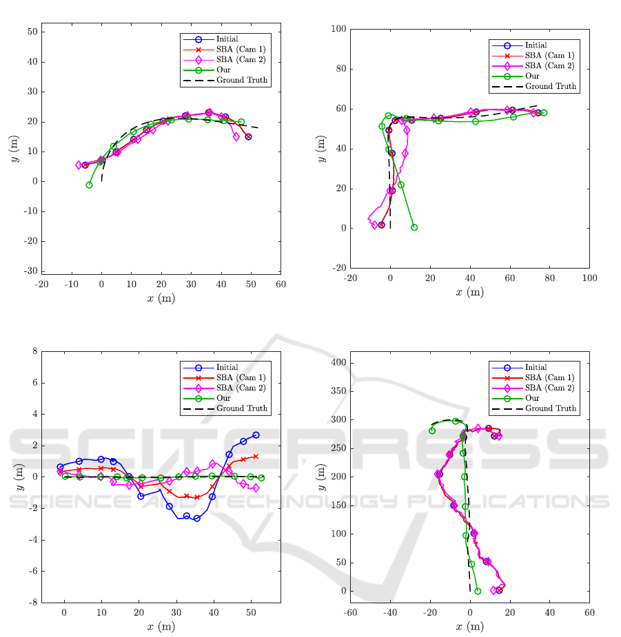
(a) Sequence 01 (60 images). (b) Sequence 03 (200 images).

Figure 3: Estimated trajectories of subsequences of Sequence 01, 03, 04 and 06. Procrustes analysis has been carried out

to align the estimated paths with the ground truth. N.B. the axes do not have the same aspect ratio in (c) in order to clearly

visualise the difference.

SLAM. IEEE Transactions on Pattern Analysis and

Machine Intelligence (PAMI), 29(6):1052–1067.

Eriksson, A., Bastian, J., Chin, T., and Isaksson, M. (2016).

A consensus-based framework for distributed bundle

adjustment. In Conference on Computer Vision and

Pattern Recognition (CVPR), pages 1754–1762, Las

Vegas, NV, USA.

Frahm, J.-M., Fite-Georgel, P., Gallup, D., Johnson, T.,

Raguram, R., Wu, C., Jen, Y.-H., Dunn, E., Clipp,

B., Lazebnik, S., and Pollefeys, M. (2010). Building

Rome on a Cloudless Day. In European Conference

on Computer Vision (ECCV), pages 368–381, Herak-

lion, Crete, Greece.

Geiger, A., Lenz, P., and Urtasun, R. (2012). Are we ready

for Autonomous Driving? The KITTI Vision Bench-

mark Suite. In Conference on Computer Vision and

Pattern Recognition (CVPR), Providence, RI, USA.

Hajjdiab, H. and Lagani

ere, R. (2004). Vision-based Multi-

Robot Simultaneous Localization and Mapping. In

Canadian Conference on Computer and Robot Vision

(CRV), pages 155–162, London, ON, Canada.

ansch, R., Drude, I., and Hellwich, O. (2016). Mod-

ICPRAM 2019 - 8th International Conference on Pattern Recognition Applications and Methods

ern Methods of Bundle Adjustment on the GPU. In

ISPRS Annals of Photogrammetry, Remote Sensing

and Spatial Information Sciences (ISPRS Congress),

pages 43–50, Prague, Czech Republic.

Hartley, R. I. and Zisserman, A. (2004). Multiple View Ge-

ometry in Computer Vision. Cambridge University

Press, Cambridge, England, UK, second edition.

Konolige, K. (2010). Sparse Sparse Bundle Adjustment.

In British Machine Vision Conference (BMVC), pages

102.1–11, Aberystwyth, Wales, UK.

Liang, B. and Pears, N. (2002). Visual Navigation using

Planar Homographies. In International Conference

on Robotics and Automation (ICRA), pages 205–210,

Washington, DC, USA.

Lourakis, M. I. A. and Argyros, A. A. (2005). Is levenberg-

marquardt the most efﬁcient optimization algorithm

for implementing bundle adjustment? In International

Conference on Computer Vision (ICCV), pages 1526–

1531, Beijing, China (PRC).

Lourakis, M. I. A. and Argyros, A. A. (2009). SBA: A

Software Package for Generic Sparse Bundle Adjust-

ment. ACM Transactions on Mathematical Software

(TOMS), 36(1):2:1–2:30.

Lowe, D. G. (2004). Distinctive Image Features from Scale-

Invariant Keypoints. International Journal of Com-

puter Vision (IJCV), 60(2):91–110.

Ort

ın, D. and Montiel, J. M. M. (2001). Indoor robot motion

based on monocular images. Robotica, 19(3):331–

342.

Scaramuzza, D. (2011a). 1-Point-RANSAC Structure from

Motion for Vehicle-Mounted Cameras by Exploiting

Non-holonomic Constraints. International Journal of

Computer Vision (IJCV), 95(1):74–85.

Scaramuzza, D. (2011b). Performance Evaluation of 1-

Point-RANSAC Visual Odometry. Journal of Field

Robotics (JFR), 28(5):792–811.

Snavely, N., Seitz, S. M., and Szeliski, R. (2008). Modeling

the World from Internet Photo Collections. Interna-

tional Journal of Computer Vision (IJCV), 80(2):189–

210.

Szeliski, R. (2011). Computer Vision: Applications and

Algorithms. Springer-Verlag, London, England, UK.

Torr, P. H. S. and Zisserman, A. (2000). MLESAC: A New

Robust Estimator with Application to Estimating Im-

age Geometry. Computer Vision and Image Under-

standing (CVIU), 78(1):138–156.

Triggs, B., McLauchlan, P. F., Hartley, R. I., and Fitzgib-

bon, A. W. (1999). Bundle Adjustment — A Modern

Synthesis. In International Workshop on Vision Al-

gorithms — Vision Algorithms: Theory and Practice,

pages 298–372, Corfu, Greece.

Valtonen

Ornhag, M. and Heyden, A. (2018a). Generaliza-

tion of Parameter Recovery in Binocular Vision for a

Planar Scene. In International Conference on Pattern

Recognition and Artiﬁcial Intelligence, pages 37–42,

Montr

eal, Canada.

Valtonen

Ornhag, M. and Heyden, A. (2018b). Rela-

tive Pose Estimation in Binocular Vision for a Pla-

nar Scene using Inter-Image Homographies. In Inter-

national Conference on Pattern Recognition Applica-

tions and Methods (ICPRAM), pages 568–575, Fun-

chal, Madeira, Portugal.

Wadenb

ack, M. and Heyden, A. (2013). Planar Motion

and Hand-Eye Calibration Using Inter-Image Homo-

graphies from a Planar Scene. In International Con-

ference on Computer Vision Theory and Applications

(VISAPP), pages 164–168, Barcelona, Spain.

Wadenb

ack, M. and Heyden, A. (2014). Ego-Motion Re-

covery and Robust Tilt Estimation for Planar Motion

Using Several Homographies. In International Con-

ference on Computer Vision Theory and Applications

(VISAPP), pages 635–639, Lisbon, Portugal.

Wu, C., Agarwal, S., Curless, B., and Seitz, S. M. (2011).

Multicore Bundle Adjustment. In Computer Vision

and Pattern Recognition (CVPR), pages 3057–3064,

Providence, RI, USA.

Zach, C. (2014). Robust Bundle Adjustment Revisited. In

European Conference on Computer Vision (ECCV),

pages 772–787, Zurich, Switzerland.

Zhang, R., Zhu, S., Fang, T., and Quan, L. (2017). Dis-

tributed very large scale bundle adjustment by global

camera consensus. In International Conference on

Computer Vision (ICCV), pages 29–38, Venice, Italy.

Zienkiewicz, J. and Davison, A. J. (2015). Extrinsics Auto-

calibration for Dense Planar Visual Odometry. Jour-

nal of Field Robotics (JFR), 32(5):803–825.

Planar Motion Bundle Adjustment