Detection of Primitives in Engineering Drawing using Genetic Algorithm

Salwan Alwan

, Jean-Marc Le Caillec

and Gerard Le Meur

Image and Information Processing, IMT Atlantique, Brest, France

Thales Group, Brest, France

Keywords:

Vectorization, Raster-to-vector Conversion, Engineering Drawings, Primitives Detection.

Abstract:

This paper presents a method for vectorizing paper drawings (raster). The method consists of skeletonizing

the input image, segmenting the skeleton based on junction detection and recognizing primitives using genetic

algorithm. The method is tested on different images and compared with previous works, results are promising

and show the high accuracy of our method.

1 INTRODUCTION

Nowadays, virtual reality (VR) and augmented reality

(AR) technologies are needed more than ever. Those

technologies are used in many environments for dif-

ferent purposes. For example, in the industrial ﬁeld,

VR and AR can be used for marketing purpose to of-

fer to the client an interactive 3D model of the prod-

uct. In addition, they can be used for training pur-

poses to teach new employs to install and repair dif-

ferent parts safely.

Paper drawings are highly available, in particu-

lar when coming to old manufactured components.

Therefore, the need for a computer-aided system con-

verting paper drawings to 3D models is essential. The

conversion from paper drawings to 3D models can be

divided into two main problems. First, raster to vec-

tor conversion, known as vectorization, which mainly

contains two sub-problems: texts/graphics separation

and primitives detection. Second, 2D drawings to 3D

models conversion.

In this paper, unlike the approaches detailed in

section 2, we propose a vectorization algorithm com-

paring primitives and selecting the best one without

extracting (remove detected pixels) or fragmenting.

This system segment skeleton using junction detec-

tion algorithm and primitive recognition using a ge-

netic algorithm by maximizing the number of pixels

of the primitive. Currently, the algorithm detects only

straight lines, circles and arcs primitives nevertheless

it can be easily extended to detect other primitives.

The outline of the paper is given as follows: Sec-

tion 2 presents related previous work of the vectoriza-

tion problem. We present in Section 3 the proposed

method of raster to vector image conversion. Section

4 describes the experimental results obtained for the

image conversion. The conclusion and some perspec-

tives of this work are given in Section 5.

2 RELATED WORKS

Image representation is classiﬁed into two categories,

raster and vector. Raster images are based on pix-

els, however, vector images are based on geometrical

shapes. The main advantage of vector images is their

ability to be scaled without affecting the resolution.

To the best of our knowledge, 3D reconstruction

algorithms C¸ ıc¸ek and G

ulesın (2004); Liu and Ye

(2005); Lee and Han (2005) have as input vector im-

ages. However, paper drawings are scanned and saved

as raster images. Thus, the aim of this paper is to pro-

pose a method to convert raster images into vectors.

Vectorization is a well-known issue in computer

vision. Several methods Dori (1997); Mandal et al.

(2010); Hilaire and Tombre (2006); De et al. (2016);

Chen et al. (1996); Song et al. (2002) have been pro-

posed to vectorize raster images for various objec-

tives. Yuan Chen et al. Chen et al. (1996) developed

RENDER which is a vectorization system showing

interesting results. However, this method is sensitive

to noise and variation of resolution. Additionally, the

inability to recreates all arcs is another weakness of

this approach. Orthogonal zig-zag Dori (1997) is a

method proposed by Dov Dori and inspired by a light

beam conducted by an optic ﬁber. This technique out-

performs the Hough transform method in terms of ex-

ecution time and vectorization results. Mandal et al.

Alwan, S., Caillec, J. and Meur, G.

Detection of Primitives in Engineering Drawing using Genetic Algorithm.

DOI: 10.5220/0007248802770282

In Proceedings of the 8th International Conference on Pattern Recognition Applications and Methods (ICPRAM 2019), pages 277-282

ISBN: 978-989-758-351-3

277

Mandal et al. (2010) vectorize horizontal and verti-

cal line segments by using mathematical morpholog-

ical tools. Also, some digital geometric properties of

straightness are used to vectorize inclined and curve

line.

One of the most interesting and robust algorithms

was done by Hilaire et Tombre Hilaire and Tombre

(2006) who used 3-4 chamfer distance for extract-

ing skeleton and maintaining all geometrical features.

By using random sampling and fuzzy primitives, the

skeleton is segmented. This method is accurate, ro-

bust to noise and precise to junction points localiza-

tion. However, this method only detects arcs and

line segments and has a high computation complex-

ity. More recently, Parmita De et al. De et al. (2016)

proposed a method called ASKME which uses also

3-4 Chamfer distance skeletonization. Parmita De et

al. propose to segment primitives by label connected

components after deleting all junctions. An adaptive

sampling method is used to detect and classify prim-

itives based on mechanical domain knowledge. This

method has several interesting features but still, Hi-

laire et Tombre method is more accurate in terms of

circle detection.

These systems yield good results, but they can

fragment primitives and decrease the accuracy of cir-

cle detection by extracting detected lines before circle

detection or fail to correctly recognize some primi-

tives which is contrary to our goal. Despite the ex-

isting systems for vectorization, there is room for im-

provement in this domain.

3 PROPOSED METHOD

The proposed method (see ﬁgure 1) aims to vector-

ize raster drawings. The algorithm uses a binarization

and a ﬁltering method to enhance the input image. It

uses (3,4) chamfer distance skeletonization algorithm

to generate the skeleton image. In addition, it uses

a junction detection algorithm to separate primitives

and a genetic algorithm to detect straight line and cir-

cles/arcs equations and endpoints. Those equations

and endpoints are used to produce vector drawings.

Figure 1: Overview of the proposed algorithm.

3.1 Preprocessing

The preprocessing step is divided into four stages: Bi-

narization, Noise Filtering, skeletonization and junc-

tion detection. The output of this algorithm is a clean

wellshaped skeleton with labeled junctions.

3.1.1 Binarization and Filtering

Due to the binary type of most source images used

to be analyzed, the binarization stage is considered

as optional. However, if the input image is not a bi-

nary image, then Otsu algorithm is used to binarize it.

Concerning the ﬁltering process, most noises gener-

ated by scanners are salt and peeper noises. A bench

of effective ﬁlters can be used for this type of noise,

we choose the median ﬁlter, which mainly replaces

each pixel with the median of neighboring entries.

3.1.2 Skeletonization and Segmentation

Skeletonization algorithms are widely used for draw-

ings vectorization. Chamfer distance skeletonization

proposed by Di Bajadi Baja (1994) is used in our

method for different reasons. First, this skeletoniza-

tion method produces a wellshaped skeleton. Sec-

ond, 3,4 chamfer distance skeletonization is robust

to noise. Moreover, this algorithm is reversible so

we can predict the original thickness of line drawing.

Those features are discussed in detail in Hilaire and

Tombre 2006.

After generating the skeleton, a junction detection

algorithm detects and label junctions of the skeleton.

The junction detection algorithm counts the detected

pixels in 8-neighbors and classiﬁes the selected pixel

based on the number of detected pixels. When the

number of detected pixels is less than two the selected

pixel is classiﬁed as an End-Point pixel. However, if

more than two pixels are detected the selected pixel is

classiﬁed as junction Arganda-Carreras et al. (2010).

A skeleton with labeled junction points is generated

and used as input for the genetic algorithm which is

explained in section 3.2.

3.2 Genetic Algorithm

A Genetic algorithm is a heuristic search method in-

spired by evolutionary biology and is widely used in

image processing and pattern recognition Lutton and

Martinez (1992); Zhang et al. (2003) ﬁelds. In this

paper, the Genetic algorithm is implemented to detect

primitives (circles/arcs and straight lines). The aim of

this method is to vectorize raster engineering draw-

ings.

ICPRAM 2019 - 8th International Conference on Pattern Recognition Applications and Methods

278

As mentioned before, the output of the previous

stages is a skeleton image whit labeled junctions. This

image is treated to generate two lists J and P where J

contains junction pixels coordinates and P contains

the rest of skeleton pixels coordinates. P is used to

generate a list CC of connected components sorted

based on their length. The longest connect compo-

nent LC is selected to be the input of the genetic al-

gorithm. An algorithm is implemented to optimize

connected components by calculating the distances

between endpoints and joining components when the

distance is smaller the threshold T HC (T H C is ob-

tained by computing the maximum length in longest

connected components in J). The genetic algorithm

generates individuals using coordinates belonging to

LC. Those individuals estimate the equation of LC

and calculate their ﬁtness function. A selection,

crossover and mutation algorithm is used to generate

new individuals. The best individual is saved and pix-

els belonging to it are deleted (The ﬁtness function

use a static copy of list P where pixels are not deleted

see section 3.2.2). In case LC is composed of several

primitives, the genetic algorithm loops until the num-

ber of pixels belonging to LC reach a certain thresh-

old T H. Each loop, the algorithm select a primitive

and update CC and LC. The algorithm loops until the

length of P reach a certain threshold T H. (see Algo-

rithm 1) The output of the algorithm is a set of solu-

tions structured as follows:

• Line solution: [m, n,c], [(x

EL1

, y

EL1

), (x

EL2

, y

EL2

)]

where (x

EL1

, y

EL1

)and((x

EL1

, y

EL1

) are the end-

points of the straight line and verifying mx +ny +

c = 0 .

• Arc solution: [(x

, y

), r], [(x

EL1

, y

EL1

), (x

EL2

, y

EL2

)]

where (x

EL1

, y

EL1

) and (x

EL1

, y

EL1

) are the end-

points of the arc and verifying (x

− x)

+ (y

−

− r

= 0.

• Circle solution:

[(x

, y

), r], [(In f , In f ), (In f , In f )] where x

, y

, r

verifying (x

− x )

+ (y

− y)

− r

= 0.

3.2.1 Individuals Generation

In this stage, we select LC from CC and use its coor-

dinates to produce individuals. A random list LI of

two different categories of individual is generated:

• Individual 1 (I1) is created by selecting two dis-

tinct points belonging to LC . These points are

used to generate the coefﬁcients of a straight

line equation. I1 is structured as follow:

{(x

, y

), (x

, y

), [m, n, c]} where (x

, y

), (x

, y

)

are the coordinates of chosen points.

Input: Raster Image

Output: Vector Output

Preprocessig;

Generating P and J list;

CC=Connected(P);

LC = CC[0];

while len(P) and len(LC) > T H do

Generate I;

Calculate F of each individual in I;

for i in range GenNb do

save Best Objective in Generation;

Generate the NewPopulation;

Calculate F of each individual in I;

Selection, Crossover, Mutation

end

Best Primitive Saved;

Update LC and P;

if len(LC) > T H then

=Connected(LC);

LC=CC

[0];

if len(LC) < T H and len(P) > T H

then

CC=Connected(P);

LC=CC[0]

end

else

if len(P) > T H then

CC=Connected(P);

LC=CC[0]

end

Algorithm 1: Vectorization Algorithm.

• Individual 2 (I2) is created by selecting three

distinct points belonging to LC. These points

are used to generate the coefﬁcients of a

circle equation. I2 is structured as fol-

low: {(x

, y

), (x

, y

), (x

, y

), [(x

, y

), r]} where

, y

), (x

, y

), (x

, y

) are the coordinates of

chosen points.

the length of LI is equal to k

and k

= k

where

and k

are respectively the length of individuals

generated of type 1 and type 2.

To summarize, we generate 50% of individuals of

type 1 and 50% individuals of type 2. Those individ-

uals are considered as solutions (equation of LC) and

they are sorted based on their Fitness Function.

3.2.2 Fitness Function

The ﬁtness or evaluation function appraises solutions

and sorts them according to the closeness to the opti-

Detection of Primitives in Engineering Drawing using Genetic Algorithm

279

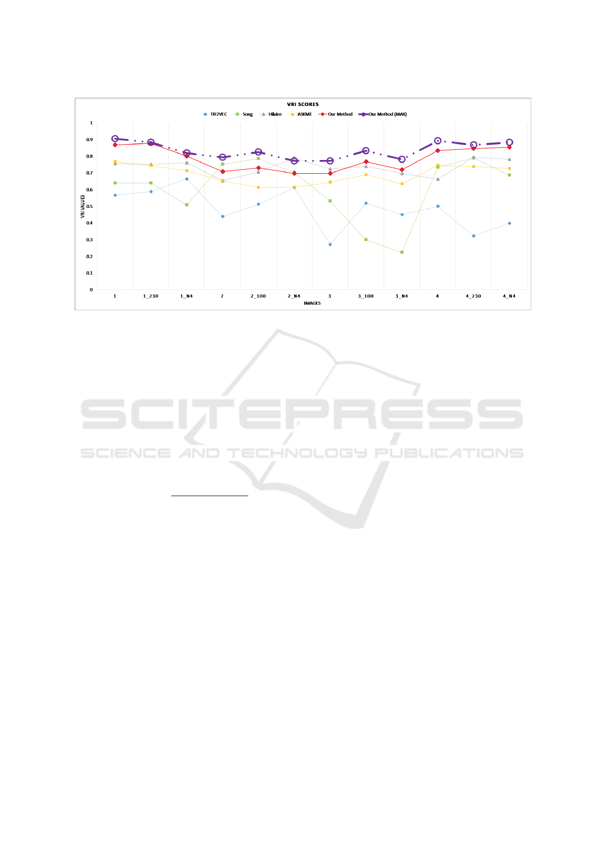
Figure 2: VRI scores comparison.

mum solution of the problem. To calculate the ﬁtness

function of each individual in I, we save all pixels in

P that belongs to the equation of each one (With tol-

erance ±1 pixel). The ﬁtness function is used to rate

individuals based on the length of a longest connected

component of detected pixels LCS (taking into con-

sideration that LCS ∩ LC 6= 0). Several equations can

detect the same length of LCS due to this tolerance.

To be more precise, we sum and average the distance

between detected pixels in LCS and the solution equa-

tion, then we subtract it from the length of LCS. The

ﬁtness function is expressed as following:

F = LLCS −

∑

i=LLCS

i=0

distance[i]

LLCS

where LLCS = length(LCS) and distance[i] is the dis-

tance between the primitive and pixel i in LCS

3.2.3 Selection, Crossover and Mutation

The selection, crossover, and mutation aim to ﬁnd the

optimal solution by converging previous solutions.

The selection algorithm used is tournament selection.

Tournament selection chooses x random individual

and then choose the best one to be a parent for the next

generation. After selecting parents, a crossover pro-

cess generates a new population by combining a ran-

dom individual with the selected parent. In addition, a

mutation variable M is used to produce new individu-

als when M < R where R is a random value between 0

and 10. Those steps allow us to converge towards the

optimal solution by generating a new population. The

following example describes the crossover process:

• Selected Parent: (x

, y

), (x

, y

)

• Generated Individual (x

, y

), (x

, y

)

• New Individual {(x

, y

), (x

, y

), [m, n, c]}

4 EXPERIMENTAL RESULTS

In this section, we present the experimental results

of our algorithm. The numbers of individuals, gen-

erations, line width, and T H are ﬁxed to 40, 50, 2

and 10 respectively. To evaluate the performance of

our method we use the Vector Recovery Index (VRI)

score Wenyin and Dori (1997) and GREC database

Liu (2003) GREC-Dataset (2003) which contains

twelve images (four original images with three dif-

ferent conditions). Figure 2 shows the VRI scores for

four previous works compared to ours. The red and

purple lines in ﬁgure 2 are the average VRI scores of

ten executions and the maximum VRI scores reached

in ten executions respectively (For more details see

table 1 in Appendix).

Figure 2 shows that our method outperforms other

methods for all images except four. However, re-

sults of those four images are promising and compet-

itive with other scores. Furthermore, maximum VRI

scores reached during ten executions outperform oth-

ers in all images except one. Moreover, our average

VRI score is the best comparing to other methods.

To the best of our knowledge, Hilaire-Tombre and

ASKME methods are producing the best results as

shown in table 1, those methods reconstruct junctions

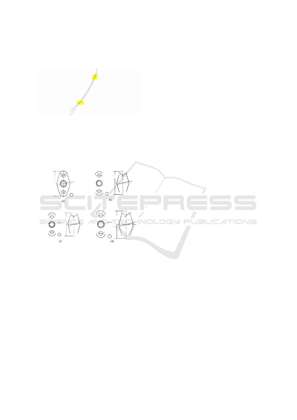
and estimates line width. As shown in ﬁgure 3, primi-

tives sometimes overlap which cause the error of end-

points detection. In addition, we ﬁxed the line width

ICPRAM 2019 - 8th International Conference on Pattern Recognition Applications and Methods

280

to 2 which affects VRI scores. Thus, by estimating

the line width and trimming primitives we expect to

improve our VRI scores.

Figure 3: Arcs intersection from vectorized image ”3”.

Based on the ﬁgure 4, we see that our algo-

rithm estimate the upper arc better than the ASKME

method and middle circles better than Hilaire-Tombre

method. To summarize, our algorithm outperforms

previous work and shows promising results. How-

ever, it needs an algorithm to unify primitives and es-

timate their width.

Figure 4: Visual comparision: (a) original image (b)

ASKME algorithm De et al. (2016) (c) Hilaire-Tombre Hi-

laire and Tombre (2006) (d) Our Method.

5 CONCLUSION AND

PERSPECTIVE

In this paper, we have presented a vectorization al-

gorithm to convert raster images into vectors. The

method is based on junction detection and genetic al-

gorithm. Our algorithm outperforms previous works

based on the VRI average score. Nevertheless, an al-

gorithm to estimate line width and solving primitives

overlapping is needed.

For the perspective of this work, we aim ﬁrst to

implement an algorithm unifying detected primitives.

Furthermore, we are looking to classify primitives and

estimate their width. Moreover, we aim to separate

dimension tools from graphics.

REFERENCES

Arganda-Carreras, I., Fern

andez-Gonz

alez, R., Mu

noz-

Barrutia, A., and Ortiz-De-Solorzano, C. (2010). 3d

reconstruction of histological sections: application to

mammary gland tissue. Microscopy research and

technique, 73(11):1019–1029.

Chen, Y., Langrana, N. A., and Das, A. K. (1996). Perfect-

ing vectorized mechanical drawings. Computer Vision

and Image Understanding, 63(2):273–286.

C¸ ıc¸ek, A. and G

ulesın, M. (2004). Reconstruction of 3d

models from 2d orthographic views using solid extru-

sion and revolution. Journal of materials processing

technology, 152(3):291–298.

De, P., Mandal, S., Bhowmick, P., and Das, A. (2016).

Askme: adaptive sampling with knowledge-driven

vectorization of mechanical engineering drawings.

International Journal on Document Analysis and

Recognition (IJDAR), 19(1):11–29.

di Baja, G. S. (1994). Well-shaped, stable, and reversible

skeletons from the (3, 4)-distance transform. Jour-

nal of visual communication and image representa-

tion, 5(1):107–115.

Dori, D. (1997). Orthogonal zig-zag: an algorithm

for vectorizing engineering drawings compared with

hough transform. Advances in Engineering Software,

28(1):11–24.

ELLIMAN, D. (2002). Tif2vec, an algorithm for arc seg-

mentation in engineering drawings. Lecture notes in

computer science, pages 350–358.

GREC-Dataset (2003). Grec’03 dataset. http:

//www.cs.cityu.edu.hk/

∼

liuwy/ArcContest/

test-images-2003.zip. Accessed: 2018-07-16.

Hilaire, X. and Tombre, K. (2006). Robust and accu-

rate vectorization of line drawings. IEEE Transac-

tions on Pattern Analysis and Machine Intelligence,

28(6):890–904.

Lee, H. and Han, S. (2005). Reconstruction of 3d interact-

ing solids of revolution from 2d orthographic views.

Computer-Aided Design, 37(13):1388–1398.

Liu, J. and Ye, B. (2005). New method of 3d reconstruction

from mechanical engineering drawings based on en-

gineering semantics understanding. In International

Conference GraphiCon’2005.

Liu, W. (2003). Report of the arc segmentation contest.

In International Workshop on Graphics Recognition,

pages 364–367. Springer.

Lutton, E. and Martinez, P. (1992). A genetic algorithm for

the detection of 2D geometric primitives in images.

PhD thesis, INRIA.

Mandal, S., Das, A. K., and Bhowmick, P. (2010). A fast

technique for vectorization of engineering drawings

using morphology and digital straightness. In Pro-

ceedings of the Seventh Indian Conference on Com-

puter Vision, Graphics and Image Processing, pages

490–497. ACM.

Song, J., Lyu, M. R., and Cai, S. (2004). Effective mul-

tiresolution arc segmentation: Algorithms and perfor-

mance evaluation. IEEE transactions on pattern anal-

ysis and machine intelligence, 26(11):1491–1506.

Detection of Primitives in Engineering Drawing using Genetic Algorithm

281

Song, J., Su, F., Li, H., and Cai, S. (2002). Raster to vec-

tor conversion of construction engineering drawings.

Automation in construction, 11(5):597–605.

Wenyin, L. and Dori, D. (1997). A protocol for performance

evaluation of line detection algorithms. Machine Vi-

sion and Applications, 9(5-6):240–250.

Zhang, L., Xu, W., and Chang, C. (2003). Genetic algorithm

for afﬁne point pattern matching. Pattern Recognition

Letters, 24(1-3):9–19.

APPENDIX

Table 1: Comparision of experimental results based on VRI.

Image Previous Methods Our Method

TIF2VEC

ELLIMAN (2002)

Song J.

Song et al. (2004)

Hilaire

Hilaire and Tombre (2006)

ASKME

De et al. (2016)

Av. Max.

1 0.567 0.641 0.756 0.769 0.869 0.906

1 230 0.589 0.64 0.752 0.745 0.878 0.883

1 n4 0.664 0.509 0.762 0.714 0.801 0.819

2 0.439 0.753 0.653 0.654 0.708 0.794

2 100 0.513 0.786 0.707 0.613 0.730 0.826

2 n4 0.612 0.703 0.791 0.615 0.697 0.772

3 0.272 0.532 0.724 0.645 0.698 0.773

3 100 0.519 0.301 0.74 0.69 0.769 0.834

3 n4 0.451 0.224 0.697 0.635 0.72 0.781

4 0.5 0.735 0.663 0.747 0.834 0.893

4 230 0.323 0.79 0.795 0.739 0.847 0.868

4 n4 0.399 0.688 0.782 0.727 0.854 0.883

Average 0.487 0.609 0.735 0.691 0.784 0.836

ICPRAM 2019 - 8th International Conference on Pattern Recognition Applications and Methods

282