
mDBSCAN: Real Time Superpixel Segmentation by DBSCAN
Clustering based on Boundary Term
Hasan Almassri
1,2
, Tim Dackermann
2
and Norbert Haala
1
1
Institute for Photogrammetry, University of Stuttgart, Germany
2
Robert Bosch GmbH Company, Reutlingen, Germany
Keywords: Clustering, Real Time, Superpixel, Segmentation.
Abstract: mDBSCAN is an improved version of DBSCAN (Density Based Spatial Clustering of Applications with
Noise) superpixel segmentation. Unlike DBSCAN algorithm, the proposed algorithm has an automatic
threshold based on the colour and gradient information. The proposed algorithm performs under different
colour space such as RGB, Lab and grey images using a novel distance measurement. The experimental results
demonstrate that the proposed algorithm outperforms the state of the art algorithms in terms of boundary
adherence and segmentation accuracy with low computational cost (30 frames/s).
1 INTRODUCTION
In these days, superpixels have a great interest in the
field of computer vision and image processing. They
have been widely applied in image segmentation
(Saito et al., 2017) (Lei, 2017) (Zhang et al., 2018),
3D reconstruction (Concha and Civera, 2014) (Kucas
and Margarita, 2017), scene flow (Vogel et al., 2013)
and object tracking (Chan et al., 2015). A superpixel
is a set of pixels that share the same features, for
example, color information, texture features, and
others. Superpixel algorithms are performed as a pre-
processing step in many computer vision applications
in order to reduce the computational time of
subsequent processing without affecting the
performance of the entire system. Therefore, fast
computation superpixel algorithms that provide high
boundary adherence and segmentation accuracy are
preferred.
Many superpixel algorithms have been introduced
such as Simple Linear Iterative Clustering (SLIC)
(Achanta et al., 2012), Entropy Rate Superpixel
Segmentation (ERS) (Liu et al., 2011)), Superpixels
Extracted via Energy-Driven Sampling (SEEDS)
(Van et al., 2012), and DBSCAN (Shen et al., 2016).
Different approaches have been followed to
generate superpixels, for example, SLIC deals with
superpixels as an iterative clustering problem. On the
other hand, SEEDS considers the superpixels as an
energy maximization problem, which achieved a
good boundary adherence. Our approach deals with
superpixels as a non-iterative clustering problem.
Moreover, it presents precisely the boundary
adherence by defining a novel simple distance
measurement that considers the boundary
information as well as the color and spatial
information between the superpixel and its neighbors.
All of the approaches are aiming to fulfill the
requirements of superpixels by having regular,
compact and connected superpixels with high
boundary adherence and low computational
complexity.
Fig. 1 shows the superpixel results of the modified
DBSCAN algorithm (mDBSCAN) that have compact
and regular shapes, which precisely represent the
image boundaries as described in section 4.5.
Recently, DBSCAN clustering algorithm (Martin et
al., 1996) has been used to generate the superpixels.
DBSCAN superpixel algorithm achieved the state of
the art algorithms at a substantially smaller
computation cost even for complex images. However,
the DBSCAN algorithm suffers from few limitations
such as it needs to be trained in order to select the
values that describe the relation between the color and
spatial information and to select the suitable threshold
value for the distance measurement. Furthermore, it
works only with RGB images. Thus, it deals with
color and spatial information, which do not perfectly
describe the boundary information.
Therefore, in this paper, we present a modified
version of the DBSCAN algorithm to overcome its
limitations as described above. The proposed
algorithm is used with introducing a novel distance
Almassri, H., Dackermann, T. and Haala, N.
mDBSCAN: Real Time Superpixel Segmentation by DBSCAN Clustering based on Boundary Term.
DOI: 10.5220/0007249302830291
In Proceedings of the 8th International Conference on Pattern Recognition Applications and Methods (ICPRAM 2019), pages 283-291
ISBN: 978-989-758-351-3
Copyright
c
2019 by SCITEPRESS – Science and Technology Publications, Lda. All rights reserved
283

measurement that enforces the connectivity and
regularity of the superpixels, which can handle gray
images as well as color images independently from
the color space. In addition, instead of training the
algorithm, our approach uses an automatic threshold
value based on color and edge information. The
proposed algorithm performs a local clustering of
pixels in 6D space for color images defined by three
color information values, one for contour information
and two values for spatial information and 4D space
for grey images defined by one color information
value, one for contour information and two values for
spatial information. mDBSCAN with low losing
meaningful image edges and low computation cost,
will be utilized as pre-processing step for optical flow
computation and moving objects tracking in a moving
platform.
The proposed algorithm has been tested on the
Berkeley segmentation benchmark . The results show
that the proposed approach outperforms the state of
the art in terms of boundary recall, under
segmentation error and explained variation.
The main contributions of this paper are:
Real time DBSCAN clustering with an automatic
parameter for distance measurement .
Novel distance measurement that works
independently from the color space such as RGB,
Lab and gray images and at the same time
improves the segmentation quality and boundary
adherence.
Figure 1: Image segmentation using mDBSCAN algorithm.
The number of superpixels are 250, 500 and 1000,
respectively.
2 RELATED WORK
In this section, we briefly revisit the DBSCAN
algorithm (Shen et al., 2016) and other important
superpixel algorithms. The superpixel algorithms are
divided into two categories: graph based algorithms
and clustering based algorithms.
2.1 Graph based Algorithms
Graph based approaches describe the image as
undirected graph consisting of vertex set and edge
weights. The vertex set represents the pixels in the
image where the edge weights define the similarities
between the neighboring pixels.
Recently, Liu et al. have proposed a graph based
algorithm .The entropy rate superpixel algorithm
(ERS) deals with superpixels as a maximization
problem. The superpixels are generated by
maximizing the entropy rate of a random walk.
According to the superpixel benchmark (Stutz et al.,
2016), ERS algorithm is one of the top performance
superpixel algorithms. It has three input parameters;
the balancing term, kernel bandwidth and the number
of superpixel. The main shortcoming of ERS
algorithm is the computation cost. As results, it needs
around 2.5 seconds to generate the superpixels for one
image which not suitable for real time applications.
2.2 Clustering based Algorithms
One of the clustering based approaches is SLIC
algorithm. In SLIC algorithm (Achanta et al., 2012),
the superpixels are generated based on a gradient
ascent principle. Firstly, initial seeds are defined
using a regular grid. After that, an iterative process is
performed to obtain better segmentation
performance. During each iteration, the seeds are
refined from the previous iteration based on the
gradient information. Because of its simplicity, low
computation cost and good boundary adherence,
SLIC becomes the most famous superpixel algorithm.
However, it has a few disadvantages. It uses an
iterative process, which increases the computation
cost. Moreover, SLIC needs a post-processing step to
enforce the connectivity (Stutz et al., 2016) (Achanta
and Süsstrunk, 2017).
On the other hand, SEEDS algorithm (Van et al.,
2012) generates the superpixels by optimizing an
energy function. Each superpixel is defined as a
region with color and shape boundary information.
Using a simple hill climbing optimization,
superpixels are refined by updating the boundaries of
the superpixels. Although the SEEDS algorithm has a
high performance in terms of boundary adherence and
computation cost, six parameters have to be defined
(Liu et al., 2011).
2.3 DBSCAN Clustering Algorithm
DBSCAN clustering algorithm (Shen et al., 2016) is
a clustering based approach for image superpixels
ICPRAM 2019 - 8th International Conference on Pattern Recognition Applications and Methods
284

segmentation by applying the density based spatial
clustering of applications with noise (DBSCAN)
algorithm. DBSCAN performs a two-steps
framework using RGB color information and spatial
information. The first step is the clustering step. In
this step, the initial superpixels are generated based
on the color information of two adjacent pixels (n, m)
using a geometric condition such that the maximu m
number of pixels in each superpixel does not exceed
a certain value as given in (2). Subsequently, the
initial superpixels are merged to form the final
superpixels through a distance measurement of both
color and spatial information of the superpixels seeds
as described in (3). DBSCAN has only one parameter
– the number of required superpixels. The authors of
the DBSCAN algorithm show that their algorithm
outperforms the state of the art and achieves the real
time capability.
(1)
(2)
(3)
Despite it has a good performance, DBSCAN
suffers from certain shortcomings. It needs to be
trained in order to select suitable parameters from (2)
and (3). The output number of superpixel per image
varies from the required number of superpixel. Lastly,
it works only under RGB images.
3 mDBSCAN ALGORITHM
Like DBSCAN, the pixels are classified into three
categories as seed, root and unlabeled sets. The top
left pixel is assigned as the first seed and root. For
each pixel in the root set, four or eight neighboring
pixels are found, then the distance between the
unlabeled pixel and both the seed pixel and root pixel
is calculated. If the unlabeled pixel satisfies the
distance measurement, it assigns the same label as the
seed pixel and considers as the next root. The process
is repeated until the termination condition such as the
searching area is satisfied. In this section, the
proposed algorithm will be described.
3.1 Contour Map
Representation of the objects boundaries in an image
is an essential property of the superpixel algorithm, as
they will be used as a pre-processing step for objects
segmentation and tracking. Therefore, the contour
map is introduced in the proposed algorithm. Given
an image I, the contour map is computed based on the
vector filed method with Sobel filter (Shinohara et al.,
1993). Firstly, the derivatives of an image are
determined, and then the maximum eigenvalues of
the Jacobian matrix J as described in (4) is computed.
The gradient value of a pixel x is computed based on
a w x w sized window around it. In this paper, w has
a value of three. The advantage of this method that no
threshold value is required and it works under all
types of color spaces. Fig. (2) shows the contour map
of an input image.
(4)
Figure 2: The contour map using the vector filed method.
3.2 Novel Distance Measurement
As explained before, the relation between an
unlabeled pixel and its seed and root is described by
a distance of color, gradient and spatial information.
The distance combines three terms i.e., normalized
spatial information, gradient information, and
weighted color information.
(5)
(6)
(7)
(8)
Where i, j, k, and G are the seed, root, unlabeled
pixel and the pixel gradient value from the contour
map, respectively. The
is the weight of the
spatial information between the seed and unlabelled
pixel. Assuming a square shape of a superpixel, each
superpixel should contain N/K pixels where N is the
total number of pixels in an image and K is the
number of required superpixels. The size of
superpixel should be control, therefore, the searching
region is restricted to an area of S x S around the seed
where S is set to be
.The
is introduced as
another geometric constraint to control the shape of
mDBSCAN: Real Time Superpixel Segmentation by DBSCAN Clustering based on Boundary Term
285

the superpixel and produce compact, regular shapes.
As given in (5), the distance measurement does not
have any external parameters; therefore, it does not
need to be trained like DBSCAN algorithm [18].
3.3 Effective Threshold Value
The main principle of DBSCAN clustering is to
compare the computed distance value with a certain
threshold. DBSCAN algorithm chooses manually the
threshold value, which adapts the value to have a
good performance. However, choosing manual
values provides scope for error especially when the
algorithm is used for real applications. This is an
important parameter where any change of its value
will affect the output of the algorithm. The proposed
algorithm introduces an automatic threshold to
compute the suitable threshold value for an input
image I. The threshold E is defined as:
Where C is the number of color channels in image
I. N describes the number of neighbors around the
pixel (it has two values 4 or 8 neighbors).
is
the standard deviation of the contour map of the
image as described in section 3.1.
3.4 Superpixel Segmentation
Algorithm
The mDBSACN consists of two steps similar to
DBSCAN algorithm; clustering step and noise
removal step. In the clustering step, the seeds are
selected in a certain order of column-by-column
(from top to bottom and from left to right). As
mentioned before, the top left pixel assigns the first
seed and root. For a seed and a root, the four or eight
neighboring pixels are obtained, then only the pixels
that fulfill the distance measurement are selected.
This step is repeated for each new combination of a
seed and a root until the searching region condition is
satisfied.
The second step is a noise removal step. Due to the
sensitivity of distance measurement and the noise in
an image, small noisy pixels are generated. DBSCAN
algorithm deals with noisy pixels indirectly as it
generates small superpixels in the first step and then
margining them to form the final superpixels.
However, using this approach will affect the number
of required superpixels as discussed in section 4.5. In
the mDBSCAN, all noisy pixels are stored in a queue
set. This queue set consists of a small group of pixels
that may not belong to the final superpixel but locate
on the searching region S x S, which will be labeled
as the final superpixel. In addition, if the small group
of pixels lies on the boundary between different
superpixels, these pixels will be considered as noisy
pixels and will be assigned a label according to the
shortest distance between these pixels and the
surrounding superpixels. All noisy pixels in the queue
set will be either root pixels or unlabeled pixels.
Algorithm 1: Superpixel clustering step.
Inputs: Image I, contour map C, regular step S.
Output: Noisy superpixel L.
for each unlabeled pixel p in image I do
set pixel p as a seed i;
find 4 or 8 neighboring pixels N
set
around seed i;
for each pixel k in N
set
do
compute the distance D
s
(i,k);
if D
k
s
(i,k) < E then
set k R
set
;
set k L(k);
endif
endfor
for each pixel k in R
set
do
if the number of pixels in L(k) < S
2
then
find 4 neighboring pixels N
set
around root j;
for each pixel m in N
set
do
compute the distance D
s
(i,j,m);
if D
s
(i,j,m) < E then
set m L(k) & set m R
set
;
else
set m
set;
endif
endfor
endif
endfor
endfor
Algorithm 2: Noise removal step.
Inputs: Superpixels L(P) and noisy superpixels Noise
set
Output: Final superpixel L
f
.
for each pixel n
s
in Noise
set
do
find the 8 neighboring superpixels N
sup
in L;
for each superpixel Q in N
sup
do
compute the distance D
s
(n
s
,Q);
endfor
find the minimum distance D
s
;
assign L(n
s
)=L(min(D
s
));
endfor
4 EXPERIMENTAL RESULTS
In this section, the proposed algorithm is compared
with four well-known and high performance state of
ICPRAM 2019 - 8th International Conference on Pattern Recognition Applications and Methods
286

the art algorithms, Superpixels Extracted via Energy-
Driven Sampling (SEEDS), Entropy Rate Superpixel
Segmentation (ERS), Simple Linear Iterative
Clustering (SLIC) and DBSCAN clustering
algorithm using the available online implementation
source codes. SEEDS and ERS are considered the
state of the art with regarding performance and SLIC
is considered the state of the in terms of computation
cost. All the methods are evaluated on the Berkeley
Segmentation Dataset 500 (BSD500). This dataset
consists of 500 images with human-labelled ground
truth segmentation. The parameters of the methods
SEEDS, ERS, SLIC, and DBSCAN are selected
according to their suggestion parameters in their
papers.
The results are demonstrated using qualitative
(visual) and quantitative comparison based on all 500
images in the BSD500 dataset, whereas DBSCAN
algorithm was evaluated based only on the testing
datasets as it needs to be trained. The qualitative
comparison is based on boundary adherence,
compactness and regularity of the superpixels as
shown in fig 5. Fig. 3 shows the results of the
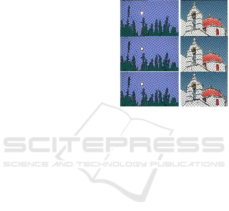
mDBSCAN based on different color space. For the
quantitative comparison as shown in fig. 4,
undersegmentation error (UE), boundary recall (Rec),
achievable segmentation accuracy (ASA) and
compactness factor (CO) are used based on the 500
images in the Berkeley Segmentation Dataset.
4.1 Undersegmentation Error (UE)
The perfect case when each superpixel overlaps with
only one object. However, sometimes the superpixel
lies on different objects that produce a segmentation
error. The undersegmentation error measures the
overlap error between the superpixel (S) and the
ground truth (G) by counting the pixels lie outside the
ground truth objects, and then divided it by the total
number of image pixels (N). The undersegmentation
error is computed using Nuebart and Protzel formulae
(Vogel et al., 2013). The lower UE value indicates
better performance.
(10)
4.2 Boundary Recall (Rec)
The boundary recall assesses the performance and
quality of boundary adherence. The boundary recall
(Rec) (Martin et al., 2004) measures the percentage
of the ground truth boundaries (G) that covered
within three pixels of a superpixel boundary (S). The
boundary recall is defined as:
(11)
Where TP (G, S) and FN (G, S) are the number of
true positive boundary pixels and the number of false
negative boundary pixels, respectively. A higher
value is better.
4.3 Achievable Segmentation Accuracy
(ASA)
The achievable segmentation accuracy computes the
highest achievable segmentation accuracy by using
superpixels as units. ASA is computed as the fraction
of the number of labeled pixels that correctly overlap
with the ground truth objects to the total number of
image pixels (Liu et al., 2011).
(12)
4.4 Compactness (CO)
The compactness is the fraction of the area of each
superpixel S to the area of a circle that has the same
perimeter of this superpixel. A higher value is better.
Schick et al. have proposed a formula to compute the
compactness as follow
(13)
4.5 Discussion of Results
A high performance superpixel algorithm is the
algorithm, which has a low undersegmentation error
with high boundary recall. Therefore,
undersegmentation error (UE), boundary recall (Rec),
achievable segmentation accuracy (ASA) and the
compactness factor (CO) are used to evaluate the
quality of the superpixel algorithms. Fig. 4 shows the
results of UE, Rec, ASA, and CO. With respect to UE,
good performance algorithm should have low UE. UE
is computed as the average value of the minimum UE
value of each image in the dataset. As shown in fig.
4a, the modified DBSCAN with lab color space
outperforms the other algorithms, whereas the other
color spaces of modified DBSCAN lie more closely
together. The reason for that is the introduction of the
contour information in the distance measurement,
mDBSCAN: Real Time Superpixel Segmentation by DBSCAN Clustering based on Boundary Term
287
which makes the edges of the superpixels overlap
consistently with the image object boundaries. For
Rec, as shown in fig. 4c, the modified DBSCAN with
lab color space achieves almost the same performance
of the SEEDS algorithm. However, the modified
DBSCAN performs better than SEEDS algorithm in
term of ASA. The modified DBSCAN has better
results than DBSCAN algorithm, as DBSCAN
algorithm generates superpixels using pre-trained
thresholds without the contour information, which
reduce the performance of the algorithm especially in
weak image boundaries as shown in fig. 5. Regarding
the compact shapes, SLIC algorithm has the most
compact and regular shapes as shown in fig. 4d.
However, the modified DBSCAN still generates
compact and regular shapes of superpixels for
different color spaces as shown in fig. 3 and fig. 5,
because of the restricted searching area as described
in section 2.2.
Another important factor for evaluating the
performance of the superpixel algorithms is the
computational cost. We perform all experiments on a
desktop PC with 32 GB RAM and 2.7GHz Intel Core
i7. According to Table 1, the computational
complexity of ERS algorithm is O(nN2logN), this
indicates that it will spend time in generating
superpixels. SLIC algorithm has a computational
complexity of O(N), however, it iterates many times
to obtain good segmentation performance and
boundary adherence.
Though the complexity of DBSCAN algorithm is
O(N), it deals with noisy pixels as small superpixels
and needs pre-trained threshold values. Our algorithm
does not need pre-trained threshold values without an
iterative process or merging step. According to the
computational time, the proposed algorithm achieves
the speed of 30fps. Thus, it is obvious that the
proposed algorithm has the real time performance.
Fig. 6 shows the computational time with regarding
to the different number of superpixels.
5 CONCLUSION
An improved real time version of DBSCAN
superpixel algorithm is introduced. Our mDBSCAN
produces regular shapes of superpixels with high
boundaries adherence in 30 fps with a novel distance
measurement. In addition, an automatic threshold is
introduced instead of using pre trained threshold
values. The mDBSCAN algorithm generates
superpixels independently of the colour space. In
future work, the proposed algorithm will be extended
to video content for tracking objects and optical flow
determination.
Figure 3: Superpixel segmentation results of the
mDBSCAN based on different color spaces. From top to
bottom, the results are obtained by using gray values, RGB
color space and lab color space.
REFERENCES
Achanta, R. and Süsstrunk, S. (2017), Superpixels and
Polygons Using Simple Non-iterative Clustering, in
'2017 IEEE Conference on Computer Vision and
Pattern Recognition (CVPR)', pp. 4895-4904.
Achanta, R.; Shaji, A.; Smith, K.; Lucchi, A.; Fua, P.and
Süsstrunk, S. (2012), 'SLIC Superpixels Compared to
State-of-the-Art Superpixel Methods', IEEE
Transactions on Pattern Analysis and Machine
Intelligence 34(11), 2274-2282.
Chan, S.; Zhou, X. and Chen, S. (2015), Online learning for
classification and object tracking with superpixel, in
'2015 IEEE International Conference on Robotics and
Biomimetics (ROBIO)', pp. 1758-1763.
Concha, A. and Civera, J. (2014), Using superpixels in
monocular SLAM, in '2014 IEEE International
Conference on Robotics and Automation (ICRA)', pp.
365-372.
http://www.mvdblive.org/seeds/
https://github.com/mingyuliutw/EntropyRateSuperpixel
https://github.com/shenjianbing/Real-time-Superpixel-
Segmentation-by-DBSCAN-Clustering-Algorithm-
https://ivrl.epfl.ch/research/superpixels
https://www2.eecs.berkeley.edu/Research/Projects/CS/visi
on/bsds/
Lei Zhou, X. H. (2017), 'Face Parsing via a Fully-
Convolutional Continuous CRF Neural Network',
arXiv.
ICPRAM 2019 - 8th International Conference on Pattern Recognition Applications and Methods
288
Table 1: The performance results of superpixel algorithms. The number of superpixel is roughly 400.
SEEDS[10]
ERS[9]
SLIC[
11]
DBSCAN[18]
mDBSCAN
Boundaries adherence
Undersegmentation error(UE)
0.152
0.128
0.143
0.132
0.109
Boundary recall (Rec)
0.923
0.775
0.727
0.792
0.923
Achievable segmentation accuracy (ASA)
0.922
0.935
0.927
0.933
0.945
Computational speed
Computational complexity
O(N)
O(nN
2
logN)
O(N)
O(N)
O(N)
Average time per image(seconds)
0.0506
0.8916
0.088
2
0.03
0.033
(a) Undersegmenation error
(b) Achievable segmentation accurracy
(c) Boundary recall
(d) Compactness factor
Figure 4: Quantitative comparison of superpixel segmentation results based on BSD500 dataset. In contrast,
undersegmentation error (lower is better), boundary recall (higher is better) and achievable segmentation accuracy (higher is
better) present the overview of the performance.
mDBSCAN: Real Time Superpixel Segmentation by DBSCAN Clustering based on Boundary Term
289
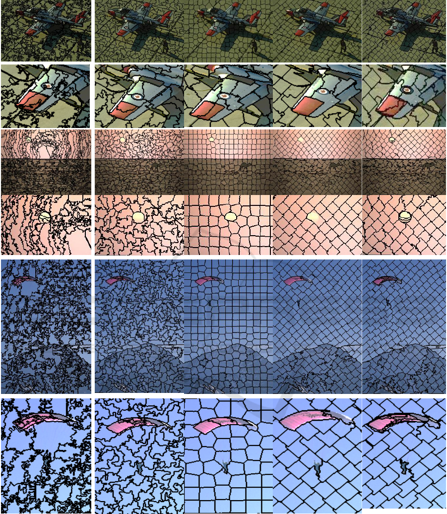
SEEDS
ERS
SLIC
DBSCAN
mDBSCAN
Figure 5: Visual comparison of superpixel segmentation results. The average number of superpixels is roughly 300.
ICPRAM 2019 - 8th International Conference on Pattern Recognition Applications and Methods
290
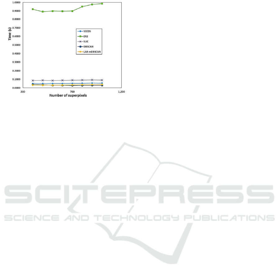
Figure 6: Computational time comparison of state of the art
superpixel algorithms (SEEDS, ERS, SLIC, DBSCAN and
mDBSCAN).
Liu, M. Y.; Tuzel, O.; Ramalingam, S. and Chellappa, R.
(2011), Entropy rate superpixel segmentation, in 'CVPR
2011', pp. 2097-2104.
Lucas, T. and Margarita, C. (2017), 'Real-time Local 3D
Reconstruction for Aerial Inspection using Superpixel
Expansion', IEEE International Conference on Robotics
and Automation.
Martin Ester, Hans-Peter Kriegel, Jörg Sander and Xiaowei
Xu (1996), A Density-Based Algorithm for Discovering
Clusters in Large Spatial Databases with Noise, in ‘
KDD'96 Proceedings of the Second International
Conference on Knowledge Discovery and Data Mining’,
pp. 226-231.
Martin, D. R.; Fowlkes, C. C. and Malik, J. (2004), 'Learning
to detect natural image boundaries using local
brightness, color, and texture cues', IEEE Transactions
on Pattern Analysis and Machine Intelligence 26(5),
530-549.
Menze, M. and Geiger, A. (2015), Object scene flow for
autonomous vehicles, in '2015 IEEE Conference on
Computer Vision and Pattern Recognition (CVPR)', pp.
3061-3070.
P.Neubert,P.Protzel, Superpixel benchmark and
comparison,in: Forum Bildverarbeitung, 2012.
Saito, S.; Kerola, T. and Tsutsui, S. (2017), 'Superpixel
clustering with deep features for unsupervised road
segmentation', arXiv.
Schick, A.; Fischer, M. and Stiefelhagen, R. (2012),
Measuring and evaluating the compactness of
superpixels, in 'Proceedings of the 21st International
Conference on Pattern Recognition (ICPR2012)', pp.
930-934.
Shen, J.; Hao, X.; Liang, Z.; Liu, Y.; Wang, W. and Shao, L.
(2016), 'Real-Time Superpixel Segmentation by
DBSCAN Clustering Algorithm', IEEE Transactions on
Image Processing 25(12), 5933-5942.
Shinohara, K.; Minami, T. and Yuki, Y. (1993), Color image
analysis in a vector field, in 'Proceedings of Canadian
Conference on Electrical and Computer Engineering',
pp. 23-26 vol.1.
Stutz, D.; Hermans, A. and Leibe, B. (2016), 'Superpixels:
An Evaluation of the State-of-the-Art', CoRR
abs/1612.01601.
Van den Bergh, M.; Boix, X.; Roig, G.; de Capitani, B. and
Van Gool, L. (2012), SEEDS: Superpixels Extracted via
Energy-Driven Sampling, in Andrew Fitzgibbon;
Svetlana Lazebnik; Pietro Perona; Yoichi Sato and
Cordelia Schmid, ed., 'Computer Vision – ECCV 2012',
Springer Berlin Heidelberg, Berlin, Heidelberg, pp. 13--
26.
Vogel, C.; Schindler, K. and Roth, S. (2013), Piecewise
Rigid Scene Flow, in '2013 IEEE International
Conference on Computer Vision', pp. 1377-1384.
Zhang, L.; Li, H.; Shen, P.; Zhu, G.; Song, J.; Shah, S. A. A.;
Bennamoun, M. and Zhang, L. (2018), 'Improving
Semantic Image Segmentation With a Probabilistic
Superpixel-Based Dense Conditional Random Field',
IEEE Access 6, 15297-15310.
mDBSCAN: Real Time Superpixel Segmentation by DBSCAN Clustering based on Boundary Term
291
