
Semantic Segmentation via Global Convolutional Network and
Concatenated Feature Maps
Chuan Kai Wang and Long Wen Chang
Department of Computer Science, National Tsing Hua University, Republic of China
Keywords: Semantic Segmentation, Convolutional Neural Network, Global Convolutional Network, DenseNet,
Concatenation, ResNet, FC-DenseNet, and CamVid.
Abstract: Most of the segmentation CNNs (convolutional neural network) based on the ResNet. Recently, Huang et
al. introduced a new classification CNN called DenseNet. Then Jégou et al. used a sequence of building
blocks for DenseNet to build their semantic segmentation CNN, called FC-DenseNet, and achieved state-of-
the-art results on CamVid dataset. In this paper, we implement the design concept of DenseNet into a
ResNet-based semantic segmentation CNN called Global Convolutional Network (GCN) and build our own
network by switching every identity mapping operation of the decoder network in GCN to a concatenation
operation. Our network uses less computational resources than FC-DenseNet to obtain a mean IoU score of
69.34% on CamVid dataset, and surpass the 66.9% obtained in the paper of FC-DenseNet.
1 INTRODUCTION
Semantic segmentation is a challenging computer
vision problem of assigning semantic labels (e.g.,
car, person, etc.) to each pixel in the given image. It
is a crucial step towards scene understanding. It
improves image classification to pixel-wise level
and could further be enhanced to instance
segmentation which distinguishes different instances
from the same semantic class. A good semantic
segmentation technique could be useful in a lot of
applications such as self-driving or other
environmental monitoring products.
In recent years, convolutional neural network
(CNN) has driven significant progression in image
classification. Networks like (Krizhevsky et al.,
2012; Simonyan et al., 2014; Szegedy et al., 2015;
He et al., 2016; Huang et al., 2017) broke the
records of many challenging benchmarks (Deng et
al., 2009; Lin et al., 2014; Krizhevsky et al., 2009)
one after another. Fully convolutional network
(FCN) (Long et al., 2015) introduced the concept of
fully convolution for replacing fully connected
layers in the last part of the classification networks
(Krizhevsky et al., 2012; Simonyan et al., 2014;
Szegedy et al., 2015). It enables these networks to
make semantic segmentation prediction under down-
sampled resolution. For up-sampling the prediction
back to original resolution, they took these
classification networks as a feature encoder network
and used the skip connection to restore the spatial
information from the feature maps in the middle
layers of the encoder network. This skip architecture
design achieved a state-of-the-art result and proved
that the pre-trained classification networks could be
extended to semantic segmentation networks.
After FCN, more and more semantic
segmentation methods (Lin et al., 2017; Peng et al.,
2017; Jégou et al., 2017) used this skip architecture
to design their own decoder networks for up-
sampling the feature maps of classification
networks. One of the methods, (Peng et al., 2015),
suggested that there still have some differences
between the principles of doing classification and
segmentation. For example, classification should be
invariant to various image transformations, but
segmentation has to be sensitive to this spatial
information. They believed that network not only
needs to use fully convolution and remove global
pooling to retain the localization information but
also has to use large convolution kernels to enhance
the capability to handle different transformations.
Following this principle, they proposed a decoder
network called Global Convolutional Network
(GCN) and achieved state-of-the-art results on
Cityscapes (Cordts et al., 2016) and Pascal-VOC
292
Wang, C. and Chang, L.
Semantic Segmentation via Global Convolutional Network and Concatenated Feature Maps.
DOI: 10.5220/0007251002920297
In Proceedings of the 8th International Conference on Pattern Recognition Applications and Methods (ICPRAM 2019), pages 292-297
ISBN: 978-989-758-351-3
Copyright
c
2019 by SCITEPRESS – Science and Technology Publications, Lda. All rights reserved

2012 (Everingham et al., 2010) datasets by using
ResNet (He et al., 2016) as thier encoder network.
In 2017, Huang et al. introduced a new
classification CNN called DenseNet where the input
of each building block is an iterative concatenation
of previous feature maps. It is similar to ResNet
which using summation through identity mapping,
but according to (Jégou et al., 2017), this small
modification brings lots of positive effects to the
network, including: (1) parameter efficiency, (2)
implicit deep supervision, and (3) feature reusing.
They used the building block of DenseNet to build
both the encoder network and the decoder network
with skip connections and named their network as
FC-DenseNet, where FC stands for fully
convolution. It used significantly fewer parameters
to achieve state-of-the-art results on CamVid
(Brostow et al., 2008) dataset without pre-training
on any dataset.
Despite the success of FC-DenseNet, we still
agree with Peng et al. that there exist additional
requirements on architecture for doing segmentation
task. We should design the decoder network based
on the principles of both DenseNet and GCN. In this
paper, we focus on utilizing the concatenation
operation to every blocks in the decoder architecture
of GCN. Therefore, we can take the advantage of
DenseNet and keep the same segmentation process
of GCN at the same time. We take reference to FC-
DenseNet and name our network as GC-DenseNet.
2 RELATED WORK
Since the size of an object in an image could be
various, semantic segmentation CNNs require
various field-of-views to recognize the objects. An
intuitive way is using multi-input to generate multi-
scale features. For example, (Chen et al., 2016) used
an attention model to decide which scale features are
more useful at each location. Another way is using
multi-path architecture to generate multi-scale
features. DeepLab (Chen et al., 2018) introduced an
“atrous spatial pyramid pooling” (ASPP)
architecture that use dilation convolutions with
different rates to create multi-scale features. As
comparison, PSPNet (Zhao et al., 2017) used a
similar architecture simply through different sizes of
pooling.
Another kind of methods is FCN-based networks
such as FC-DenseNet (Jégou et al., 2017) and GCN
(Peng et al., 2017), which reused the feature maps in
the encoder network to obtain multi-scale field-of-
views. FC-DenseNet tried to implement dense block
(Huang et al., 2017) in their decoder network.
Unlike other FCN-based methods using pre-trained
classification network, they re-built the encoder with
five dense blocks according to their own
combination. Finally, they built the decoder
symmetrical to the encoder. Since the number of
feature map channels increase each time through a
building block, it will be computationally expensive
for the decoder network. They did not transfer
previous feature maps to the next dense block during
up-sampling. However, we think it violates the
principle of DenseNet and causes their network
could not improve further.
GCN is the network we reference the most. It
took pre-trained ResNet as the encoder network and
used global convolutional networks to extract
classification features from the encoder network. It
is constructed by 2 pairs of and
convolution layers with different orders where k is
an editable kernel size. To further refine the
prediction around object boundary, they added
boundary refinement blocks after each GCN block
and up-sampling layer. They set the output channels
of every blocks in the decoder network to the
number of semantic classes. Each GCN block would
learn to make a segmentation prediction under
different field-of-views.
3 METHOD
To present our method, we will introduce the
overview of our semantic segmentation network in
section 3.1. Then, in section 3.2, we will explain the
architecture details of each block in our network.
3.1 Overview
Since our network is based on the architecture of
GCN (Peng et al., 2017), we take architecture figure
in their paper as reference to draw the overview of
our network in Figure 1. In Figure 1(a), we show the
overview of our network architecture. The leftmost
column is a DenseNet (Huang et al., 2017) without
the classification layer. It is our encoder network.
The rest of the blocks construct our decoder
network. Each output feature map of a “dense block”
(DB) is transferred through a “global convolution”
(GC) block and a “boundary refinement” (BR)
block. Then the feature map with lower resolution is
up-sampled by a “transposed convolution layer”
(TC) and concatenated (Concat.) with the higher
resolution one. After a sequence of up-sampling, the
last feature map is passed to the final BR block.
Semantic Segmentation via Global Convolutional Network and Concatenated Feature Maps
293
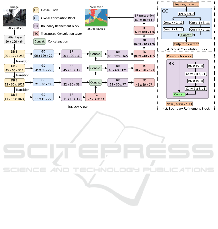
Figure 1: Architecture of our network. (a) Overview of the whole network. (b) Global convolution block architecture. (c)
Boundary refinement block architecture.
It abandons the previous feature maps and generates
a score map with 11 channels corresponding to 11
semantic classes in the CamVid dataset (Brostow et
al., 2008). Finally, the prediction of each pixel label
is determined to be the class with the highest score.
3.2 Architecture Details
Unlike ResNet down-sampling the feature maps at
the first convolution layer in each ResNet block,
DenseNet implements it at the transition layers. We
replace the ResNet in GCN with DenseNet and skip
connect the output feature maps of each dense block
to our global convolution block before transition
layers.
Our main modification of the decoder network in
GCN is switching every identity mapping operation
to a concatenation operation. To make each block
act more like a building block for DenseNet, we add
the batch normalization (Ioffe et al., 2015) and
ReLU (Nair et al., 2010) before of global
convolution blocks and the convolution layers in
boundary refinement blocks. Since there always has
a batch normalization after the convolution layer, we
remove the bias operation in every convolution
layers.
As for up-sampling layer, we use transposed
convolution (Noh et al., 2010) with 33 kernel and
stride 2. Due to concatenation operations, the
number of feature map channel will not remain the
same like GCN does. Thus we remove the
concatenation in the last boundary refinement block.
It only outputs the new feature map with channel
equals to the number of semantic classes.
4 EXPERIMENTAL RESULTS
In this section, we will first introduce the training
details of our network in section 4.1. Then, we
conduct several experiments with different network
settings in section 4.2 to find the best result of our
network. Finally, we compare our best setting
network with other networks in section 4.3.
We use “mean intersection of union” (mIoU) to
measure the performance. The mIoU of every
semantic classes “” are computed by:
,
(1)
where
,
, and
denotes the number of
pixels belong to “true positive”, “false positive”, and
“false negative” of the prediction on class “ ”.
Therefore, the score value will be always between
0%~100%, and the higher is the better.
4.1 Training Details
We use PyTorch (Paszke et al., 2017) to implement
our network models. We evaluate our network
performance on CamVid (Brostow et al., 2008)
dataset. It is a 360480 urban scene video frame
ICPRAM 2019 - 8th International Conference on Pattern Recognition Applications and Methods
294
dataset which consists of 367 frames for training,
101 frames for validation, and 233 frames for
testing. Each frame is fully labelled with 11
semantic classes and a void class.
We add dropout layers with 0.2 dropping rate
after each block in the decoder network and the
building blocks in the DenseNet. All models are
trained on data augmented with random horizontal
flips and normalization on RGB channels.
We initialize our models using HeUniform (He
et al., 2015) and train them using Adam (Kingma et
al., 2014) with 175 epochs and a batch size of 4. We
set the initial learning rate of 10
-4
and multiply it by
0.4 at epoch 125 and 150. Finally, we regularize our
model with a weight decay of 10
-4
. All of our
network trainings run on a Nvidia GTX 1080 GPU
with 8GB memory.
4.2 Finding the Best Setting
Since DenseNet (Huang et al., 2017) has different
depth version pre-trained on ImageNet (Deng et al.,
2009), we want to find the best suit version for our
network. We use the same size of global convolution
kernel (k=7) to train our network with different
DenseNet depth in Table 1. The results show that
DesneNet-121 is the best choice for our network on
CamVid dataset. We believe it is because that
CamVid is a dataset much smaller than ImageNet
comparing to the number of classes and data. It does
not need that many parameters to solve the problem.
Then we need to find the best kernel size of
global convolution kernel. Based on the above
experiment, we use DesneNet-121 and transposed
convolution to build our network with different
global convolution kernel size k in Table 2. In
contrast to Peng et al. finding k =15 is the best size
on Pascal-VOC 2012 (Everingham et al., 2010), we
get the best result at k = 7 on CamVid instead. We
think the reason is that CamVid dataset does not
contain any object with the full image size like
Pascal-VOC 2012.
Table 1: Comparison of DenseNet depth on CamVid
testing dataset.
Depth = 121
Depth = 169
Depth = 201
mIoU (%)
69.34
69.03
69.14
Table 2: Comparison of global convolution kernel size on
CamVid testing dataset.
k = 3
k = 7
k = 11
k = 15
mIoU (%)
68.87
69.34
68.61
67.77
Table 3: Comparison of GCN and our network.
GCN-ResNet
GCN- DenseNet
ours
mIoU (%)
64.15
64.69
69.34
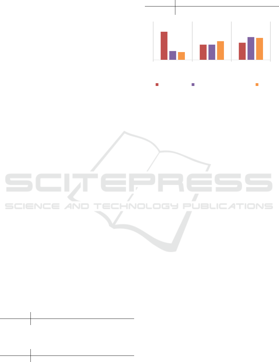
Figure 2: Computational efficiency for GCN-ResNet, FC-
DenseNet, and ours.
Hence we do not need a kernel with the full size of
the final output feature map of encoder network.
4.3 Comparing to Other Networks
Since (Peng et al., 2017) only evaluate GCN on
Pascal-VOC 2012 (Everingham et al., 2010) and
Cityscapes (Cordts, 2016), we have to implement the
network and evaluate it on CamVid (Brostow et al.,
2008) by ourselves. Additionally, we hope to
distinguish our contribution of modifying the
decoder network from simply replacing the ResNet
with the DenseNet. Therefore, we also build a
DenseNet version of GCN, which only switch the
encoder network without doing any modification on
the decoder network. We denote this model as GCN-
DenseNet and compare these two versions of GCN
to our network in Table 3. All the networks uses
77 global convolution kernels. The results show
that DenseNet really is better than ResNet in
semantic segmentation task. However, the difference
is not that obvious. On the contrary, our
modification of the decoder network does contribute
most of the improvement because we use
concatenation to provide more flexibility for the
feature combination.
Since DenseNet use much fewer parameters than
ResNet, we will not just compare the computational
efficiency to GCN-ResNet. We also compare our
network with FC-DenseNet. In Figure 2, we
compare the number of training parameters, training
time of each epoch, and the consumption of GPU
memory on GCN-ResNet, FC-DenseNet, and our
network. All the networks are trained with batch size
of 4. Unlike GCN-ResNet, ours is trained with full
size images, while FC-DenseNet is only trained with
58.77
40
4497
9.32
40
5961
8.21
49
5731
# Parameters
(Milion)
Training Time
(Sec/Epoch)
GPU Memory
(MB)
GCN-ResNet FC-DenseNet (224 x 224) Ours
Semantic Segmentation via Global Convolutional Network and Concatenated Feature Maps
295
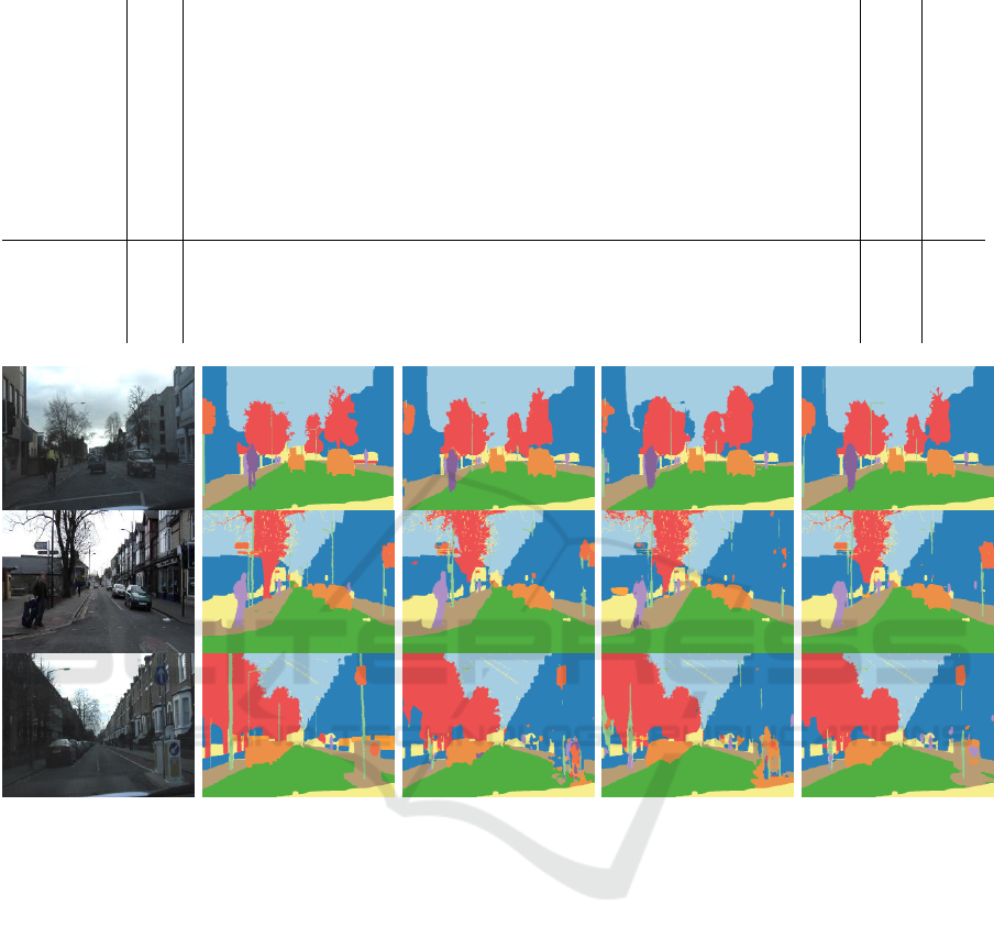
Table 4: Comparison of our and other networks in each class IoU (%).
Model
# parameters (M)
Sky
Building
Pole
Road
Sidewalk
Tree
Sign
Fence
Car
Pedestrian
Cyclist
mIoU (%)
Pixel Accuracy (%)
FC-DenseNet
9.32
90.92
81.93
35.34
95.22
83.60
75.56
43.32
36.93
80.51
57.20
45.15
65.97
91.27
GCN-ResNet
58.77
91.56
82.70
26.45
93.76
78.95
76.11
40.08
36.67
82.79
50.15
46.39
64.15
90.96
GCN-DenseNet
7.42
91.50
83.61
30.46
94.93
84.04
76.09
37.66
39.98
78.12
51.36
43.79
64.69
91.53
GC-DenseNet
8.21
92.32
84.71
35.91
94.69
82.15
77.06
46.69
46.22
84.86
56.15
61.94
69.34
92.14
(a) Input
(b) Ground Truth
(c) GCN-ResNet
(d) FC-DenseNet
(e) Our method
Figure 3: Comparison of our method and other methods.
224224 random cropped patches.
Although GCN-ResNet uses much more
parameters, it takes less GPU memory and trains
faster than our network, because FC-DenseNet and
our network use more channels of the feature maps
in the decoder network. As for FC-DenseNet, it uses
slightly more parameters and memory than ours. The
only downside of our network is it trains slower than
other networks, because it has more channels in the
decoded feature maps with higher resolution. In
Figure 3, we show our results is better than GCN-
ResNet and ) FC-DenseNet in detail such as the
sign pole in the image.
In Table 3, we show each semantic class IoU
separately and mIoU of each network. We also
compute the pixel accuracy to see how many pixels
are predicted correctly. Despite GCN-DenseNet is
our experimental network, our GC-DenseNet use the
least number of parameters and achieve the highest
mIoU score. Our network brings improvement on
almost every classes, especially those classes with
low mIoU score.
5 CONCLUSION
In this paper, we propose a semantic segmentation
CNN that modifies the GCN-ResNet (Peng et al.,
2017) with concatenation architecture introduced in
DenseNet. Although our network takes more GPU
memory comparing to GCN-ResNet, it uses fewer
parameters and achieves the mIoU score higher than
GCN-ResNet and FC-DenseNet in CamVid dataset.
In contrast to DenseNet-264 obtaining a
classification accuracy close to the ResNet-152, we
ICPRAM 2019 - 8th International Conference on Pattern Recognition Applications and Methods
296

simply use DenseNet-121 in GCN-DenseNet to
achieve the mIoU score better than GCN-ResNet,
which use ResNet-152 as the encoder network. It
shows that concatenation architecture is more
suitable than identity mapping architecture for
semantic segmentation.
REFERENCES
Krizhevsky, A., Sutskever, I., Hinton, G. E., 2012.
ImageNet classification with deep convolutional
neural networks. In Conference on Neural Information
Processing Systems, pp. 1097-1105.
Simonyan, K., Zisserman, A., 2014. Very deep
convolutional networks for large-scale image
recognition. In arXiv preprint arXiv: 1409.1556.
Szegedy, C., Liu, W., Jia, Y., Sermanet, P., Reed, S.,
Anguelov, D., Erhan, D., Vanhoucke, V., Rabinovich,
A., 2015. Going deeper with convolutions. In IEEE
Conference on Computer Vision and Pattern
Recognition, pp. 1-9.
He, K., Zhang, X., Ren, S., Sun, J., 2016. Deep residual
learning for image recognition. In IEEE Conference on
Computer Vision and Pattern Recognition, pp. 770-
778.
Huang, G., Liu, Z., Maaten, L. van der, Weinberger, K.
Q., 2017. Densely connected convolutional networks.
In IEEE Conference on Computer Vision and Pattern
Recognition, pp. 2261-2269.
Deng, J., Dong, W., Socher, R., Li, L. J., Li, K., Li, F. F.,
2009. ImageNet: A large-scale hierarchical image
database. In IEEE Conference on Computer Vision
and Pattern Recognition, pp. 248-255.
Lin, T. Y., Maire, M., Belongie, S., Bourdev, L., Girshick,
R., Hays, J., Perona, P., Ramanan, D., Zitnick, C. L.,
Dollár, P., 2014. Microsoft COCO: Common objects
in context. In European Conference on Computer
Vision, pp. 740-755.
Krizhevsky, A., Hinton, G. E., 2009. Learning multiple
layers of features from tiny images. In Tech Report,
University of Toronto.
Long, J., Shelhamer, E., Darrell, T., 2015. Fully
convolutional networks for semantic segmentation. In
IEEE Conference on Computer Vision and Pattern
Recognition, pp. 3431-3440.
Lin, G, Milan, A., Shen, C., Reid, I., 2017. RefineNet:
Multi-path refinement networks for high-resolution
semantic segmentation. In IEEE Conference on
Computer Vision and Pattern Recognition, pp. 5168-
5177.
Peng, C., Zhang, X., Yu, G., Luo, G., Sun, J., 2017. Large
kernel matters -- Improve semantic segmentation by
global convolutional network. In IEEE Conference on
Computer Vision and Pattern Recognition, pp. 1743-
1751.
Jégou, S., Drozdzal, M., Vazquez, D., Romero, A.,
Bengio, Y., 2017. The one hundred layers tiramisu:
Fully convolutional DenseNets for semantic
segmentation. In IEEE Conference on Computer
Vision and Pattern Recognition, pp. 1175-1183.
Everingham, M., Gool, L. V., Williams, C. K. I., Winn, J.,
Zisserman, A., 2010. The PASCAL visual object
classes (VOC) challenge. In International journal of
computer vision, pp. 303-338.
Cordts, M., Omran, M., Ramos, S., Rehfeld, T.,
Enzweiler, M., Benenson, R., Franke, U., Roth, S.,
Schiele, B., 2016. The cityscapes dataset for semantic
urban scene understanding. In IEEE Conference on
Computer Vision and Pattern Recognition, pp. 3213-
3223.
Brostow, G. J., Shotton, J., Fauqueur, J., Cipolla, R., 2008.
Segmentation and recognition using structure from
motion point clouds. In European Conference on
Computer Vision, pp. 44-57.
Chen, L. C., Yang, Y., Wang, J., Xu, W., Yuille, A. L.,
2016. Attention to scale: Scale-aware semantic image
segmentation. In IEEE Conference on Computer
Vision and Pattern Recognition, pp. 3640-3649.
Chen, L. C., Papandreou, G., Kokkinos, I., Murphy, K.,
Yuille, A. L., 2018. DeepLab: Semantic image
segmentation with deep convolutional nets, atrous
convolution, and fully connected CRFs. In IEEE
Transactions on Pattern Analysis and Machine
Intelligence, pp. 834-848.
Zhao, H., Shi, J., Qi, X., Wang, X., Jia, J., 2017. Pyramid
scene parsing network. In IEEE Conference on
Computer Vision and Pattern Recognition, pp. 2881-
2891.
Ioffe, S., Szegedy, C., 2015. Batch normalization:
Accelerating deep network training by reducing
internal covariate shift. In International Conference on
Machine Learning, pp. 448-456.
Nair, V., Hinton, G. E., 2010. Rectified linear units
improve restricted boltzmann machines. In
International Conference on Machine Learning, pp.
807-814.
Noh, H., Hong, S., Han, B., 2015. Learning deconvolution
network for semantic segmentation. In Proceedings of
the IEEE International Conference on Computer
Vision, pp. 1520-1528.
Paszke, A., Gross, S., Chintala, S., Chanan, G., Yang, E.,
DeVito, Z., Lin, Z., Desmaison, A., Antiga, L., Lerer,
A., 2017. Automatic differentiation in PyTorch.
He, K., Zhang, X., Ren, S., Sun, J., 2015. Delving deep
into rectifiers: Surpassing human-level performance
on ImageNet classification. In Proceedings of the
IEEE International Conference on Computer Vision,
pp. 1026-1034.
Kingma, D. P., Ba, J. L., 2014. Adam: A method for
stochastic optimization. In arXiv preprint
arXiv:1412.6980.
Semantic Segmentation via Global Convolutional Network and Concatenated Feature Maps
297
