
Colorization of Grayscale Image Sequences using Texture Descriptors
Andre Peres Ramos and Franklin Cesar Flores
Departamento de Informatica, Universidade Estadual de Maringa, Maringa, Brazil
Keywords:
Colorization, Segmentation, Tracking.
Abstract:
Colorization is the process of adding colors to a monochromatic image or video. Usually, the process involves
to segment the image in regions of interest and then apply colors to each one, for videos, this process is repeated
for each frame, which makes it a tedious and time-consuming job. We propose a new assisted method for video
colorization, the user only has to colorize one frame and then the colors are propagated to following frames.
The user can intervene at any time to correct eventual errors in the color assignment. The method consists
of extract intensity and texture descriptors from the frames and then perform a feature matching to determine
the best color for each segment. To reduce computation time and give a better spatial coherence we narrow
the area of search and give weights for each feature to emphasize texture descriptors. To give a more natural
result we use an optimization algorithm to make the color propagation. Experimental results in several image
sequences, compared to others existing methods, demonstrates that the proposed method perform a better
colorization with less time and user interference.
1 INTRODUCTION
Colorization is the process of add colors to monochro-
matic images and videos. Although colorization ap-
pears to be a recent process, there are registries da-
ting from 1.842 and possibly early (Yatziv and Sapiro,
2006), making the processes as old as photography
itself. However, even now, with digital images, the
process is extremely tedious, costly and slow. The
manual process consist in the user manually to seg-
ment all object of interest in regions, then assign a
color to each region of image until reach the desired
result, for videos this steps are repeated for all frames
until all of them are colored.
Because of the process complexity, several met-
hods addresses the colorization problem in attempt
to reduce the amount of work involved. However,
the number methods that addresses video colorization
is very small compared to those that addresses sta-
tic image, perhaps because of its complexity and high
processing cost(Paul et al., 2017).
Broadly, the state-of-the-art colorization methods
for videos and images, in the literature, can be divi-
ded in two big classes: assisted colorization methods
and automatic colorization methods. Mostly of as-
sisted methods (Levin et al., 2004), (Yatziv and Sa-
piro, 2006), (Qu et al., 2006), (Luan et al., 2007),
(Irony et al., 2005), (Huang et al., 2005), (Hyun et al.,
2012), (Paul et al., 2017), are based on work of Levin
et al(Levin et al., 2004), they require that the user put
marks in the image using colored scribbles, then the
algorithm propagates the colors from these scribbles
to the whole image. The major problem with scribbles
oriented methods are that they usually require many
user interventions, where the user has to add a high
number of scribbles to archive a good result. Some
methods like (Luan et al., 2007; Qu et al., 2006) uses
texture descriptors in order to reduce the amount of
scribbles, others, as (Yatziv and Sapiro, 2006) aims
the reduction of processing time.
The automatic methods (Zhang et al., 2016; Ii-
zuka et al., 2016; Bugeau et al., 2014; Gupta et al.,
2012), (Irony et al., 2005) perform the colorization
without any user input. Some (Gupta et al., 2012;
Irony et al., 2005), (Bugeau et al., 2014) uses similar
images, provided by the user, as reference, to make
the color transfer; others (Zhang et al., 2016; Iizuka
et al., 2016) utilizes Convolution Neural Networks
(CNN). The networks are trained using a set of ima-
ges, after reached some accuracy level, it is used to
guess the color of a given grayscale image. Both au-
tomatics approaches have limitations residing on the
fact that there are ambiguity when determining the co-
lor of a grayscale image.
Although these methods have good results in sta-
tic images, none of them has proved to be efficient
for videos, in order to reduce the work and time spent
Ramos, A. and Flores, F.
Colorization of Grayscale Image Sequences using Texture Descriptors.
DOI: 10.5220/0007252203030310
In Proceedings of the 14th International Joint Conference on Computer Vision, Imaging and Computer Graphics Theory and Applications (VISIGRAPP 2019), pages 303-310
ISBN: 978-989-758-354-4
Copyright
c
2019 by SCITEPRESS – Science and Technology Publications, Lda. All rights reserved
303

in the colorization process while maintaining a good
visual result. The use of assisted image colorization
methods in videos require that the user repeats the en-
tire process for each frame, which ends up making the
process time consuming and tiring. In its turns, auto-
matic image colorization methods does not perform
well in videos, since it treats each frame individually,
it is possible that the same object receive different co-
lors in two frames which will cause artifacts in the
final result.
In this paper, we propose a novel assisted colo-
rization method for grayscale videos that the user,
through a tool developed for this purpose, perform the
colorization of the first frame, according to his taste.
After that, texture and intensity descriptors are extrac-
ted from the frames to carry out the color propagation
from the manually colored frame to the following fra-
mes, the user can intervene at any time, correcting any
errors in the process or adding colors to new objects
in the scene. Automating part of the process while gi-
ving full control to the user on the desired result, ea-
sily solving common problems in video colorization
such as occlusion and scene changes.
2 PROPOSED COLORIZATION
METHOD
The proposed method colorizes a sequence of images
through the matching of texture, intensity and region
features between two consecutive frames of the same
sequence. The user only has to fully colorize a first
frame, even so, using a tool made to speed up the pro-
cess thought an interactive segmentation method, like
Watershed segmentation. Then, the method automati-
cally transfer color from the first frame to the second
using feature matching. The user can interact with the
result, approving or making the desired changes, ap-
plying new colors or change the designated ones, after
that, the process repeats using the new colored frame
as reference to colorize the next one, these steps con-
tinue until all frames are fully colorized.
We can split our method in six stages: (a) seg-
mentation, (b) manual colorization of the first frame,
(c) feature extraction, (d) feature matching, (e) color
transfer and propagation, and (f) user evaluation and
interference.
2.0.1 Algorithm
For a best understand of out proposed method we des-
cribe a simple implementation of it in algorithm 1
which demonstrate the simplicity of the presented so-
lution.
Let be E ⊂ Z × Z a rectangular finite subset of
points and x ∈ E one of these points. Let K = [0, k] be
a totally ordered set. Denote by Fun[E, K] the set of
all functions f : E → K, a grayscale image is one of
these functions.
Let C
i
: E → Chr the chrominance information of a
colored image where Chr = a × b and a = [−1, ..., 1],
b = [−1, ..., 1], being a the green to red light intensity
and b the blue to yellow color intensity, according to
CIE L*a*b* color space.
Let I : {I
1
, I
2
, ..., I
n
} : I
i
∈ Fun[E, K] be the original
grayscale image sequence.
Let C : {C
1
, C
2
, ..., C
n
} : C
i
∈ Fun[E, Chr] be the
set of chrominance information for sequence S and
O : {O
1
, O
2
, ..., O
n
} : O
i
→ Chr ×K the final colorized
image.
Let S the segmented I sequence, being S
i
the frame
I
i
but segmented by an automatic segmentation algo-
rithm and r a segment from S
i
.
Let U (i, r, rad) = {r
j
: ∃x ∈ r
j
: DE(x, CP(r)) ≤
rad} be the set of all segments from S
i−1
that has
points within a predetermined radius rad from the
center coordinates of segment r ∈ S
i
. Where r
j
∈
S
i−1
, DE(x, CP(r)) is the euclidean distance between
a point x and CP(r) being CP(r) the center point of a
segment r.
Let FD
r
(t) a function that computes the sum of
the weighted distances between the features of seg-
ments t and r.
Let MD
i
(r) = t ∈ S
i−1
: FD
r
(t) = min
j
{FD
r
(t
j
) :
t
j
∈ U(i, r, rad)} the function that will return the best
matching from the candidates segments for the seg-
ment r.
Let segment(I) be a function that perform an au-
tomatically segmentation for every frame I
i
. Let be
Propagate(I
i
, C
i
) a function that perform the final co-
lor propagation through the usage of the algorithm
proposed in (Levin et al., 2004).
The details of all these functions will be described
in the following sections.
2.1 Segmentation
We start the process using a super-segmentation algo-
rithm on the image set I to generate the segmented set
S, in order to break down every frame in smalls seg-
ments. We need to use a super-segmentation method
that make segments enough to properly separate the
objects in the scene, but, at the same time, make regi-
ons big enough to extract relevant texture descriptor,
give a good spatial coherency, a homogeneous result
and avoid an excessive processing.
In ours experiments, we utilize the Superpixel seg-
mentation algorithm, also called as Superpixel repre-
VISAPP 2019 - 14th International Conference on Computer Vision Theory and Applications
304

Algorithm 1: Algorithm for the proposed method.
Input - Grayscale image sequence I
Output - Colored image sequence
O
S ← segment(I)
for all segment r ∈ S
1
do
//User manually colorize the frame S
1
define chrominance (a,b) for region r : a ∈ a, b ∈
b;
C
1
(x) ← (a, b), ∀x ∈ r;
end for
for i in [2..n] do
for all segment r in S
i
do
t ← MD
i
(r);
C
i
(x) ← C
i−1
(y), ∀x ∈ r, y ∈ t;
end for
//User can change the colors of segments in C
i
O
i
← Propagate(I
i
, C
i
);
end for
sentation. As the algorithm group adjacent similar
pixel based on a predetermined grid, it avoids very
small and insignificant regions as give control on how
many regions it is desired. We utilize SEEDS Super-
pixel implementation(Van den Bergh et al., 2012) in
ours experiments. As parameters, we use 5,000 for
the number of Superpixel, 4 for the Number of Levels
and 10 Iterations.
2.2 Manual Colorization of First Frame
For the method to be able to colorize the sequence, an
initial a color information is necessary, this informa-
tion is provided by a colored frame, usually the first
frame of the sequence.
As our goal is to colorize monochromatic image
sequences, normally, there are no prior color infor-
mation available, so we ask the user to colorize an
initial frame. The manual colorization of even of a
single frame, without any assisted method, is a time-
consuming process and demand a lot of work. The-
refore, we develop a simple tool to assist the segmen-
tation process. We utilize an implementation of wa-
tershed segmentation algorithm(Vincent and Soille,
1991; Vincent, 1992) using markers. Through this
tool, the user create custom regions and assign colors
to it, the user also can freely colorize the image ma-
king strokes, where each region r of the image that is
touched by the stroke will receive the selected color.
2.3 Feature Extraction
One of the most important stage of the method is to
extract descriptive features to get good matching re-
sult. In our method, we use three distinct features,
generating a 101-dimensional feature vector by each
Superpixel segment, composed of a 2-dimensional in-
tensity vector, a 40-dimensional Gabor Feature vector
and a 59-dimensional LBP histogram used as texture
descriptor feature. These features are computed as
follow:
2.3.1 Intensity
The two-dimensional intensity feature is extracted for
each segment, the first dimension is composed by the
simple average of pixels intensities belong to the seg-
ment. The second dimension is computed by the sim-
ple average of intensity of all pixels belong to the
neighbor segments.
For a frame i, be n the number of pixel in segment
r and I
i
(x) the intensity of pixel x, the first dimension
is computed by equation 1.
FI
i
(r) =
1
n
∑
x∈r
I
i
(x) (1)
For the second dimension, be M the number of
neighbors segments from r, be r
k
a neighbor segment
and N(r) the set of r’s neighbor segments, the feature
can be computed by equation 2.
FN
i
(r) =
1
M
∑
r
k
∈ N(r)
FI
i
(r
k
) (2)
2.3.2 Gabor Features
The Gabor Features (Manjunath and Ma, 1996) are
widely used as texture descriptor in processing of di-
gital images, it has a special characteristic that it can
analyze texture information in both space and fre-
quency domain, also it was based in the behavior of
the visual cortex neurons(Yang et al., 2003). The ex-
traction occurs through the creation of filters that are
applied in a convolution process in the image; the re-
sult of the process is the Gabor Feature Bank. We
use 40 different filter composed of eight orientati-
ons, varying from 0 to 7π/8 and five exponential sca-
les exp(i ∗ π), i=[0,1,2,3,4], then the feature value for
each dimension of a segment is computed as the sim-
ple average of Gabor feature value for all pixel in the
segment.
Let be G the set of all Gabor features for the whole
segmented image S
i
, let G
d
be a dimension of Gabor
feature for the image, G
d
(x) the value of feature bank
for the point x. The Gabor Feature for a segment r and
the dimension d can be computed by equation 3, the
process is applied to all dimensions G
d
in G to form
the 40-dimension feature vector.
Colorization of Grayscale Image Sequences using Texture Descriptors
305

FG
i
(r, G
d
) =
1
n
∑
x∈r
G
d
(x) (3)
2.3.3 Local Binary Pattern
Local Binary Pattern (LBP) is another texture des-
criptor widely used in image and signal proces-
sing, is highly descriptive and has a low processing
cost (Ahonen et al., 2006). Usually, it is used the his-
togram of LBP’s result as texture descriptor. In our
case, to compute a feature vector for a segment S
i
,
we compute the histogram of LBP’s result but only
for the values within the segment. As parameters, we
use a radius of 1 and 8 as the number of neighboring
points, we use the uniform calculation.
Because the uniform LBP can have N(N − 1) + 3
possible values, begin N the number of neighboring
points, we can have up to 59 values with our current
parameters, therefore, 59 positions in the histogram
with make our 59-dimension LBP vector for each seg-
ment.
2.4 Feature Matching
2.4.1 Search Area
The extracted features are used to find the best match
between the segments of the reference frame and the
segments of frame to be colorized. The color from
the best matching segment is used in the colorization
process.
To reduce the amount of processing time, as well
as give a better spatial coherence, we narrow the com-
parison area within a predetermined radius from the
borders of the region to be colorized.
Given a segment to be colorized r and U(i, r, rad)
the set of candidate segments from the reference
frame S
i−1
to use in the matching process with r. We
must find a x ∈ r point that is in the center of segment
area, then we find U(i, r, rad) segments by choosing
only the segments in S
i−1
that has pixel inside an area
formed by a radius rad from the center point x in S
i−1
,
we use the euclidean distance to compute the distance
between two points. We summarize this process in
equation 4 where DE(x, y) stands for the euclidean
distance between two points and CP(r) for the center
point of segment r.
U(i, r, rad) = {r
j
: ∃x ∈ r
j
: DE(x, CP(r)) ≤ rad}
(4)
With this, we narrow down the search area for
only the segments in U(i, r, rad) which will not only
reduce the number of comparisons but will also main-
tain a spatial coherence avoiding computations with
far segments.
2.4.2 Matching
With the candidates segments found in the previous
subsection for a segment S
i
to be colorized, we must
find the best match among these segments to extract
the color from it. To find the best match, we calcu-
late the shortest distance between features vectors, for
each feature.
We use Cityblock distance to calculate the distance
between two features vector, this distance has a lower
computational cost compared to others, like euclidean
distance. The distance is calculated by the equation 5
where a and b are two feature vector with n dimension
each.
D(a, b) =
n
∑
j=1
a
j
− b
j
(5)
As we use three different features to classify, we
must set weights to each one, once texture features
is more descriptive for us than intensity feature. For
each type of feature, is calculated the distance bet-
ween features of the segment to be colorized and from
the candidates segments. These distances are nor-
malized, multiplied by a weight and summed giving
a unique distance value for each candidate segment.
The segment with the lowest value will be the match.
In ours experiments, we use the following weights:
0.20 for intensity, 0.45 for LBP and 0.35 for Gabor
features.
Let r denote the segment to be colorized from
frame i and u one of the candidates segment from the
set U(i, r, rad) of the already colored reference frame
S
i−1
, we want to find the segment u with the lowest
FD
r
(u) value, that is, the lowest sum of the weighted
distances between the features of segments t and r.
The normalization and weighting is expressed in
equations 6 and 7 where W
k
is the weight value for
feature k and D
k
(r, u) the distance between the seg-
ments r and u for a feature k. The final FD
r
(u) value
for a segment is computed by equation 8.
T
k
(r) =
∑
z∈U (i,r,rad)
D
k
(r, z) (6)
Λ
r,k
(u) =
D
k
(r, u)
T
k
(r)
W
k
(7)
FD
r
(u) =
∑
k
Λ
r,k
(u) (8)
2.5 Color Transfer and Propagation
Once it is found matches for all segments, the co-
lor transfer starts, we work with CIE L*a*b* color
VISAPP 2019 - 14th International Conference on Computer Vision Theory and Applications
306
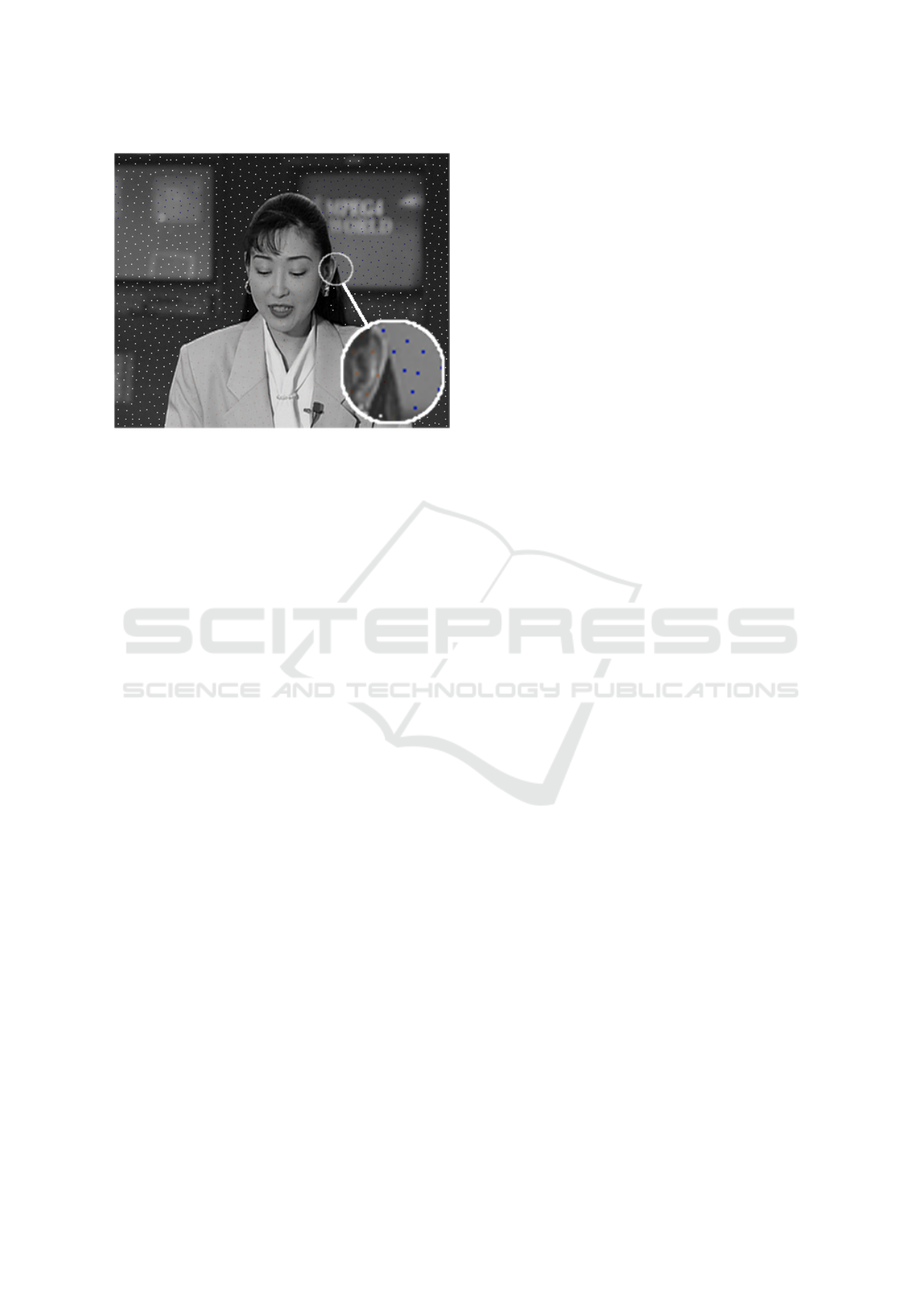
Figure 1: Micro-scribbles for the color propagation.
space, where L* stands for lightness or intensity, a*
for the green to red and b* blue to yellow color lights.
As a grayscale image only have the intensity chan-
nel we only have to transfer the a* and b* to fulfill the
color information. However a direct transfer maybe
not produce a good result, once that gradual chan-
ges in luminance often indicates a gradual transition
in chrominance in natural images (Yatziv and Sapiro,
2006; Kimmel, 1998).
To produce a more realistic result, instead of fill
the entire segment with chrominance value from the
best match, we create micro-scribbles of only one
pixel in the center of to be colorized segment, these
micro-scribbles are shown in figure 1.
The micro-scribbles are then propagate to all ot-
her pixel; to do a smooth propagation we use an op-
timization algorithm. The algorithm is based on the
principle that neighbor pixels with similar luminance
must also have similar color, more details about algo-
rithm is presented in Levin’s et al work (Levin et al.,
2004).
2.6 User Evaluation and Interference
After each segment has an assigned color, we give to
the user the option to analyze and, if he wants, inter-
vene in the result, changing the color of some regions.
For that, we create a simple tool where a preview of
the results it is showed to the user, he can select a co-
lor, or use one already present in the image, and apply
this color to the segments of the frame. Once the user
is satisfied with the result, the final frame is generated
and the user can analyze the next one.
3 EXPERIMENTS
All experiments were performed in an Intel i7-6700
3.40GHz CPU PC with 8GB of ram memory, the met-
hod was implemented in Python 2.7 language with
OpenCV, Numpy and SciPy packages. The image
sequence that are originally colored had it color in-
formation removed before the experiments. For the
algorithms used in comparison (Larsson et al., 2016;
Zhang et al., 2017; Gupta et al., 2017) we use the aut-
hors provided implementation.
We created a Graphical User Interface (GUI) for
each tested method. These GUIs are also used to col-
lect data regarding the time and interference.
3.1 Evaluation
For our work, we used three metrics to evaluate, there
are: (a) processing time and user’s interference per
frame, (b) segmentation error and (e) Color Peak Sig-
nal to Noise Ratio (CPSRN) the details of each one
will be described in the following subsection.
3.1.1 Processing Time and User’s Interference
per Frame
Once the goal of our method is to reduce time and
work in the colorization process, one evaluation is to
measure how less work and time it consumes in com-
parison with other methods.
For our method, we compute the total time per
frame as the time that the method takes to segment,
extract the features, and perform the comparisons and
the designation of the colors. Plus the time that the
user takes to analyze, apply their modification and re-
quest the next frame, the interference per frame num-
ber is computed as the total of times that user changes
the color of a segment.
For the manual method, the total time is computed
as the time that user takes to segment, assign color to
each region and request the next frame. For interfe-
rence, is computed as the total of times that user add
or remove a segment and assign a color to a region.
For the other methods, the total time is calculated
as the time the user takes to add, modify and remove
scribbles (when necessary) and process each frame.
For the interference, the total of operations to add, re-
move or modify scribbles.
3.1.2 Segmentation Error
As the colorization can be defined as a sub-problem
of segmentation, a measure for the segmentation can
be used as an indication of the quality of the result.
Colorization of Grayscale Image Sequences using Texture Descriptors
307

For compute the segmentation error, we used a
modified version of method proposed in (Flores and
de Alencar Lotufo, 2010) because instead of have
only foreground and background object we have se-
veral objects as the image has one region for each area
with different color.
As we use a super-segmented image, to be possi-
ble to compare with a ground truth, we have to group
adjacently segments that have the same chrominance
information creating big single-colored regions.
Let Z
i
be the set of z
m
regions, such that z
m
is a
union of r ∈ S
i
segments. A region r ∈ S
i
belongs
to z
m
∈ Z
i
if exists a r
2
∈ Z
i
such that r and r
2
are
adjacent and C
i
(x) = C
i
(y), x ∈ r, y ∈ r
2
Let m
v
be the binary segmentation mask for a re-
gion v from the segmentation Z
i
, where 1 indicates
that the pixel belongs to the region and 0 otherwise.
And let g
v
be the ground truth segmentation mask for
the same region. Being ψ the symmetrical difference
between m
v
and g
v
, given by
ψ(m
v
, g
v
) =
(
1 if |m
v
− g
v
| = 1,
0 otherwise
(9)
We compute the segmentation error SE(Z
i
) for a
segmentation Z
i
as the average of all regions errors
by equations 10 and 11 where #(m
v
) stands for the
number of pixels valued 1 in a binary mask m
v
. We
divide the error of each region by 2 to avoid duplicate
computation of the same error, as an error in a region
will be also an error in the adjacent region.
ER(m
v
) =
#(ψ(m
v
, g
v
))
#(m
v
) + #(g
v
)
(10)
SE(Z
i
) =
1
n
n
∑
v=1
ER(m
v
)
2
(11)
3.1.3 Color Peak Signal to Noise Ratio
CPSNR provide a relative evaluation of colorization
techniques, CPSNR is evaluated as the average mean
square error of R, G and B color channels to measure
the distortions in the color channels from a ground-
truth (Pang et al., 2014; Paul et al., 2017). Given two
8-bit color images I
1
and I
2
of the same dimensions
H ×W the CPSNR can be computed as equations 12
and 13, the result is measured in Decibels (dB) where
the higher the value the better the result.
MSE =
1
3HW
∑
Ω∈(R,G,B)
H
∑
i=1
W
∑
j=1
(I
(Ω)
1
(i, j) − I
(Ω)
2
(i, j))
(12)
CPSNR = 10 log
10
255
2
MSE
(13)
Table 1: Average Colorization Time per Frame.
Sequence
Time-per frame (s)
Larsson
et al.,
2016
Zhang
et al.,
2017
Gupta
et al.,
2017
Manual Proposed
Foreman 7.50 291 195 333.05 34.02
Akiyo 7.3 275 183 310.52 33.43
Carphone 7.5 254 180 319.79 26.16
Table 2: Average CPSNR values per frame.
Sequence
Average CPSNR per frame frame (dB)
Larsson
et al.,
2016
Zhang
et al.,
2017
Gupta
et al.,
2017
Manual Proposed
Foreman 30.41 31.51 31.63 32.87 32.93
Akiyo 29.28 31.78 32.46 33.11 33.17
Carphone 29.58 31.03 31.71 32.51 32.69
3.2 Results
In the experiments presented in this paper we utilize
three image sequences already known in the digital
image processing community they are Foreman Se-
quence, Akiyo Sequence and Carphone Sequence, we
utilize the first 150 frames of each sequence.
Although these sequence are originally colored,
we removed the colors working purely on grayscale
version, was necessary to use sequence that already
had colors to be able to calculate the CPSNR, however
this method is intended to be used in native grayscale
sequences. We apply our method in all three sequence
using the evaluation described in previous subsecti-
ons.
For a comparison of our method, we made the co-
lorization of the same frames using a manual method,
we also compare with methods proposed in (Larsson
et al., 2016; Zhang et al., 2017), (Gupta et al., 2017)
and we made the adaptation for video colorization
proposed by the authors, using Lukas-Kanade opti-
cal flow method to estimate scribbles motion between
frames.
The results are shown in tables 1, 2 and 3. We
also show the segmentation error for our method in
table 4, as the methods proposed in (Larsson et al.,
2016; Zhang et al., 2017), (Gupta et al., 2017) do not
threat the problem as a segmentation problem we was
unable to make a comparison, we do not calculated
the segmentation error for the manual method because
to colorize the user performs what he understands to
be optimal segmentation.
The results show that our method is faster than the
manual implementation and requires less interference
by the user. In addition, the CPSNR value for our met-
hod is a little better than the manual, this occurs be-
cause the manual method does not provide a smooth
VISAPP 2019 - 14th International Conference on Computer Vision Theory and Applications
308
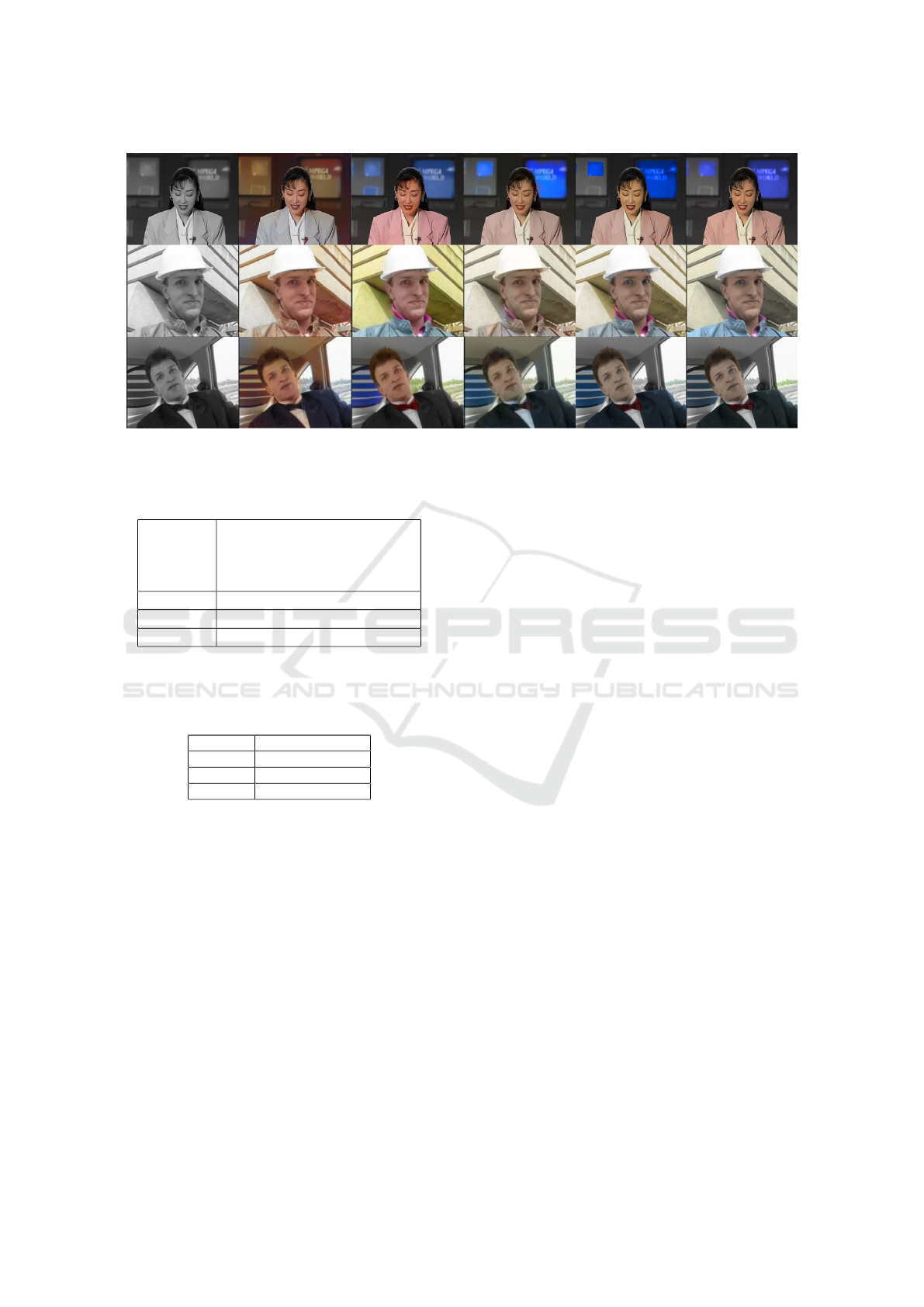
Figure 2: Comparison of the proposed method results with the methods proposed in (Larsson et al., 2016; Zhang et al.,
2017; Gupta et al., 2017) and manual method, for frame 100 of Akiyo, Foreman and Carphone sequences. From the left, the
grayscale original image, (Larsson et al., 2016), (Zhang et al., 2017), (Gupta et al., 2017), manual and the proposed Method.
Table 3: Average User’s interference per frame.
Sequence
User’s Interference Per Frame
Zhang
et al.,
2017
Manual Proposed
Foreman 51.54 51.75 7.59
Akiyo 46.94 41.08 7.22
Carphone 37.14 70.01 10.77
obs: This metric cannot be apllied to Larsson et al., 2016 and
Gupta et al., 2018, once they are fully automated methods.
Table 4: Average Segmentation error compared to the
Ground-Thruth.
Sequence Segmentation Error
Foreman 3.34%
Akiyo 3.31%
Carphone 2.51%
color transition between regions.
In comparison with other methods in the literature,
the proposed method shown to be faster, this occurs
because these methods demands to previous manually
colorize several frames to achieve a good result, also
has an additional computation time to calculate opti-
cal flow to each scribble.
For the CPSNR values the proposed method has
slightly better values for most of cases, again we be-
lieve that this occurs because of optical flow, as the
quality deteriorates between frames until reach the
next already colorized frame, for the interference per
frame also has better values for our methods in most
of the cases.
The proposed method also achieve a low segmen-
tation error compared to the ground truth, it is impor-
tant to remember that sometimes there is subjectivity
about ideal segmentation, so achieving a perfect re-
sult is impractical. Thus, we consider the error value
acceptable for the problem, taking into consideration
that the method does not directly transfer the colors,
but rather does a propagation, which makes small seg-
mentation errors often imperceptible to the result.
The visual result for the frame number 100 of all
sequences is shown in figure 3, for all methods, the
actual frame had not user interference, begin the last
interference only in previous frame.
4 CONCLUSIONS
In this paper, we present a method for the colorization
of grayscale images sequences, using texture descrip-
tors to perform color transfer between frames. The
user only have to manually colorize one first frame,
even though with the help of an assisted segmentation,
the user can intervene at any time to correct possible
errors. .
Experiments shows that our method significantly
reduce the time and interventions needed to achieve
good results in comparison with others methods in the
literature. Although some methods presented smaller
times, the quality of the result was well inferior to the
proposed method. The segmentations errors compa-
red to a manually generated ground truth is very low
taking in account that the methods segmentation is ge-
nerated automatically and it uses a color propagation
algorithm.
We also compute the CPSNR between the real
color and color provided by the methods, our met-
hod had better values for state-of-the-art methods and
even for the manual colorization, since it make a color
Colorization of Grayscale Image Sequences using Texture Descriptors
309

blending providing a more realistic result. In future
work, we suggest the experiment of others descriptor
that may give an even more descriptive result, as well,
other methods of feature comparison.
ACKNOWLEDGEMENTS
We would like to thank the Instituto Federal do Pa-
rana - IFPR for releasing the first author of his work
activities, allowing the development of this research.
REFERENCES
Ahonen, T., Hadid, A., and Pietikainen, M. (2006). Face
description with local binary patterns: Application to
face recognition. IEEE transactions on pattern analy-
sis and machine intelligence, 28(12):2037–2041.
Bugeau, A., Ta, V.-T., and Papadakis, N. (2014). Variational
exemplar-based image colorization. IEEE Transacti-
ons on Image Processing, 23(1):298–307.
Flores, F. C. and de Alencar Lotufo, R. (2010). Watershed
from propagated markers: An interactive method to
morphological object segmentation in image sequen-
ces. Image and Vision Computing, 28(11):1491–1514.
Gupta, R. K., Chia, A. Y.-S., Rajan, D., Ng, E. S., and
Zhiyong, H. (2012). Image colorization using similar
images. In Proceedings of the 20th ACM international
conference on Multimedia, pages 369–378. ACM.
Gupta, R. K., Chia, A. Y.-S., Rajan, D., and Zhiyong,
H. (2017). A learning-based approach for automa-
tic image and video colorization. arXiv preprint
arXiv:1704.04610.
Huang, Y.-C., Tung, Y.-S., Chen, J.-C., Wang, S.-W., and
Wu, J.-L. (2005). An adaptive edge detection based
colorization algorithm and its applications. In Pro-
ceedings of the 13th annual ACM international confe-
rence on Multimedia, pages 351–354. ACM.
Hyun, D.-Y., Heu, J.-H., Kim, C.-S., and Lee, S.-U. (2012).
Prioritized image and video colorization based on
gaussian pyramid of gradient images. Journal of Elec-
tronic Imaging, 21(2):023027.
Iizuka, S., Simo-Serra, E., and Ishikawa, H. (2016). Let
there be color!: joint end-to-end learning of global and
local image priors for automatic image colorization
with simultaneous classification. ACM Transactions
on Graphics (TOG), 35(4):110.
Irony, R., Cohen-Or, D., and Lischinski, D. (2005). Co-
lorization by example. Proceedings of the Sixteenth
Eurographics conference on Rendering Techniques.
Kimmel, R. (1998). A natural norm for color processing. In
Asian Conference on Computer Vision, pages 88–95.
Springer.
Larsson, G., Maire, M., and Shakhnarovich, G. (2016).
Learning representations for automatic colorization.
In European Conference on Computer Vision, pages
577–593. Springer.
Levin, A., Lischinski, D., and Weiss, Y. (2004). Colori-
zation using optimization. In ACM Transactions on
Graphics (ToG), volume 23, pages 689–694. ACM.
Luan, Q., Wen, F., Cohen-Or, D., Liang, L., Xu, Y.-Q., and
Shum, H.-Y. (2007). Natural image colorization. In
Proceedings of the 18th Eurographics conference on
Rendering Techniques, pages 309–320. Eurographics
Association.
Manjunath, B. S. and Ma, W.-Y. (1996). Texture features
for browsing and retrieval of image data. IEEE Tran-
sactions on pattern analysis and machine intelligence,
18(8):837–842.
Pang, J., Au, O. C., Yamashita, Y., Ling, Y., Guo, Y., and
Zeng, J. (2014). Self-similarity-based image coloriza-
tion. In Image Processing (ICIP), 2014 IEEE Interna-
tional Conference on, pages 4687–4691. IEEE.
Paul, S., Bhattacharya, S., and Gupta, S. (2017). Spatio-
temporal colorization of video using 3d steerable py-
ramids. IEEE Transactions on Circuits and Systems
for Video Technology, 27(8):1605–1619.
Qu, Y., Wong, T.-T., and Heng, P.-A. (2006). Manga co-
lorization. In ACM Transactions on Graphics (TOG),
volume 25, pages 1214–1220. ACM.
Van den Bergh, M., Boix, X., Roig, G., de Capitani, B., and
Van Gool, L. (2012). Seeds: Superpixels extracted via
energy-driven sampling. In European conference on
computer vision, pages 13–26. Springer.
Vincent, L. (1992). Recent developments in morphological
algorithms. ACTA STEREOLOGICA, 11:521–521.
Vincent, L. and Soille, P. (1991). Watersheds in digital spa-
ces: an efficient algorithm based on immersion simu-
lations. IEEE Transactions on Pattern Analysis & Ma-
chine Intelligence, (6):583–598.
Yang, J., Liu, L., Jiang, T., and Fan, Y. (2003). A
modified gabor filter design method for fingerprint
image enhancement. Pattern Recognition Letters,
24(12):1805–1817.
Yatziv, L. and Sapiro, G. (2006). Fast image and video
colorization using chrominance blending. In IEEE
transactions on image processing, volume 15, pages
1120–1129. IEEE.
Zhang, R., Isola, P., and Efros, A. A. (2016). Colorful image
colorization. In European Conference on Computer
Vision, pages 649–666. Springer.
Zhang, R., Zhu, J.-Y., Isola, P., Geng, X., Lin, A. S., Yu, T.,
and Efros, A. A. (2017). Real-time user-guided image
colorization with learned deep priors. arXiv preprint
arXiv:1705.02999.
VISAPP 2019 - 14th International Conference on Computer Vision Theory and Applications
310
