Deep Learning for Radar Pulse Detection

Ha Q. Nguyen, Dat T. Ngo and Van Long Do

Viettel Research and Development Institute, Hoa Lac High-tech Park, Hanoi, Vietnam

Keywords:

Deep Neural Network, Radar Pulse Detection, Radar Pulse Parameter Estimation, Pulse Description Word,

Change Point Detection, Pruned Exact Linear Time.

Abstract:

In this paper, we introduce a deep learning based framework for sequential detection of rectangular radar

pulses with varying waveforms and pulse widths under a wide range of noise levels. The method is divided

into two stages. In the ﬁrst stage, a convolutional neural network is trained to determine whether a pulse

or part of a pulse appears in a segment of the signal envelop. In the second stage, the change points in the

segment are found by solving an optimization problem and then combined with previously detected edges to

estimate the pulse locations. The proposed scheme is noise-blind as it does not require a noise ﬂoor estimation,

unlike the threshold-based edge detection (TED) method. Simulations also show that our method signiﬁcantly

outperforms TED in highly noisy cases.

1 INTRODUCTION

The detection of radar pulses—or the estimation of

the times of arrival (TOAs) and the times of departure

(TODs)—plays a central role in passive location sys-

tems as it provides input for other algorithms to locate

the emitter (Torrieri, 1984; Poisel, 2005). This is a

challenging task since radar pulses are modulated and

coded with a variety of waveforms and most of the

time buried in noise. Existing methods for radar pulse

detection are usually threshold-based (Torrieri, 1974;

Iglesias et al., 2014) in which the thresholds are deter-

mined via an estimation of the noise statistics. These

methods work well with high or moderate Signal-to-

Noise-Ratios (SNRs) but perform poorly with low

SNRs. Furthermore, the noise ﬂoor estimation—a

prerequisite of these algorithms—is itself a hard prob-

lem, especially in highly varying environments.

In the past few years, Deep Learning (LeCun

et al., 2015; Goodfellow et al., 2016) has proved

a powerful tool for many tasks in computer vi-

sion and signal processing, notably, image classiﬁca-

tion (Krizhevsky et al., 2012; Szegedy et al., 2015; He

et al., 2016) and object detection (Ren et al., 2017;

Redmon et al., 2016; Liu et al., 2016). Motivated

by these successes, we propose a novel method for

radar pulse detection in which edges are sequentially

estimated from segments of the received signal en-

velop via a deep-learning-based segment classi-

ﬁcation followed by a ﬁnd-change-points algorithm

(Killick et al., 2012). The segment classiﬁcation es-

sentially determines if a pulse is present, partially

present, or absent in a segment through a Convo-

lutional Neural Network (CNN). For a segment of

small-enough length, it can only fall into one of the

5 categories: ‘2 edges’, ‘TOA only’, ‘TOD only’, ‘All

pulse’, and ‘All noise’. Based on the output of the

CNN, the ﬁnd-change-points routine seeks edges in

the segment by minimizing a cost function associated

to the number of edges, instead of a thresholding pro-

cedure. This approach is therefore able to get rid of

the unreliable noise ﬂoor estimation. The contribu-

tions of our paper are summarized as follows.

 A novel CNN architecture for segment classiﬁca-

tion.

 An algorithm for adaptive segment classiﬁcation

in which the CNN predicts the class of the current

segment based on the conﬁdence of its previous

prediction.

 An algorithm for sequential pulse localization

that combines the segment classiﬁcation with

a ﬁnd-change-points algorithm. This method

signiﬁcantly surpasses the performance of the

Threshold-based Edge Detection (Iglesias et al.,

2014), especially in the low-SNR regimes.

The rest of the paper is outlined as follows: Sec. 2

formulates the problem. Sec. 3 constructs the CNN

and integrates it into an adaptive algorithm for seg-

ment classiﬁcation. Sec. 4 presents the main algo-

Nguyen, H., Ngo, D. and Do, V.

Deep Learning for Radar Pulse Detection.

DOI: 10.5220/0007253000320039

In Proceedings of the 8th International Conference on Pattern Recognition Applications and Methods (ICPRAM 2019), pages 32-39

ISBN: 978-989-758-351-3

rithm for sequential pulse localization. Sec. 5 reports

some numerical results. Finally, Sec. 6 provides con-

cluding remarks.

2 PROBLEM FORMULATION

In this paper, we are interested in the detection

of radar pulses in a narrow bandwidth of, say,

78.125 MHz, centered at frequency 0.

Assuming

Nyquist sampling, we acquire a discrete-time cor-

rupted signal

ˆx[n] = x[n] + w[n], n ∈ Z, (1)

where x is a complex-valued signal that contains a

train of rectangular pulses and w is an additive white

Gaussian noise (AWGN). Note that, each sample of

the discrete-time signal then corresponds to a period

of 12.8 ns. The pulses might have various wave-

forms and pulse widths. We consider in this pa-

per 7 types of pulse modulations that are commonly

used in modern radar systems (Levanon and Moze-

son, 2004; Richards, 2014; Pace, 2009), namely, Con-

tinuous Waveform (CW), Step Frequency Modulation

(SFM), Linear Frequency Modulation (LFM), Non-

Linear Frequency Modulation (NLFM), Costas code

(COSTAS), Barker code (BARKER), and Frank code

(FRANK). See Fig. 1 for an illustration of these mod-

ulations. The pulse widths vary in an extremely large

range from about 0.1 µs to about 400 µs, which corre-

sponds to a range from 8 samples to 31250 samples.

The location of each pulse is characterized by

the time of arrival (TOA)—the middle of the rising

edge—and the time of departure (TOD)—the middle

of the falling edge. Our task is to estimate the series

of TOAs and TODs in an sequential manner by look-

ing at one segment of the noisy signal ˆx at a time. To

reduce the effect of noise, we perform a preprocess-

ing step in which a lowpass ﬁlter h of bandwidth 20

MHz is applied to ˆx to get

ˆx

= h ∗ ˆx = h ∗ x + h ∗ w =: x

+ w

, (2)

where w

is now a color Gaussian noise. Our detec-

tion algorithm takes as input sequential segments of

the envelop (or magnitude) | ˆx

| and outputs a list of

pulse description words (PDWs), each of which con-

sists of a TOA and a TOD of the corresponding pulse.

This is done via a CNN-based adaptive classiﬁcation

of the segments followed by a ﬁnd-change-points al-

gorithm that will be described in the next sections.

In practice, the detection of radar pulses would involve

a frequency tuning from wide band to narrow band. This

crucial step is out of the scope of this paper and will be

discussed elsewhere.

0 5 10 15 20 25

Time (us)

0.2

0.4

0.6

0.8

(a) CW

0 5 10 15 20 25

Time (us)

0.2

0.4

0.6

0.8

(b) SFM

0 5 10 15 20 25

Time (us)

0.2

0.4

0.6

0.8

0 5 10 15 20 25

Time (us)

0.2

0.4

0.6

0.8

(d) NLFM

0 5 10 15 20 25

Time (us)

0.2

0.4

0.6

0.8

(e) COSTAS

0 5 10 15 20 25

Time (us)

0.2

0.4

0.6

0.8

(f) BARKER

0 5 10 15 20 25

Time (us)

0.2

0.4

0.6

0.8

(g) FRANK

Figure 1: Envelops of 7 modulation types of rectangu-

lar pulses without noise. What shown here are the results

achieved after the 20-MHz-lowpass ﬁltering.

3 CNN-BASED SEGMENT

CLASSIFICATION

From a practical point of view, we can reasonably as-

sume that the distance between consecutive pulses is

at least 30 µs, which is equivalent to about 2344 sam-

ples. Therefore, we choose to divide the envelop | ˆx

into segments of k = 2000 samples with 50% overlap-

ping.

This is to make sure that there will be at most

one pulse in a segment. Then, each segment can only

fall into one of the following 5 classes.

• Class 1 (‘2 edges’): a TOA and a TOD of a pulse

both appear in the segment.

• Class 2 (‘TOA only’): a TOA appears in the seg-

ment without TOD.

• Class 3 (‘TOD only’): a TOD appears in the seg-

ment without TOA.

• Class 4 (‘All pulse’): the whole segment is part of

a long pulse.

• Class 5 (‘All noise’): the segment contains only

background noise.

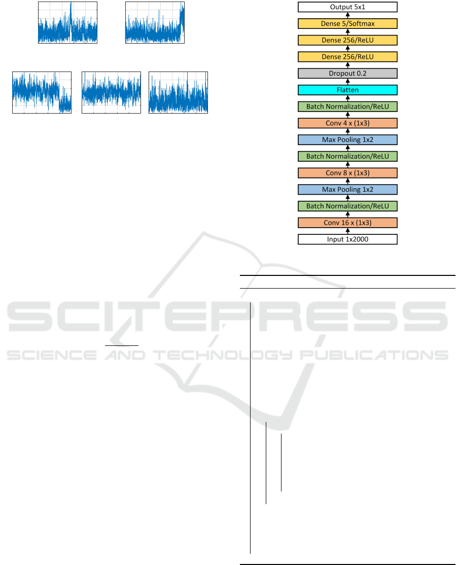
Fig. 2 depicts these classes under a relatively low

SNR. To perform the segment classiﬁcation, we pro-

pose a Convolutional Neural Network (CNN) whose

architecture is shown in Fig. 3. This network consists

of 13 hidden layer, including 3 convolution layers and

3 dense layers. Each convolution layer is followed

In general, the segment length should be chosen to be

equal to the minimum distance between consecutive pulses.

Deep Learning for Radar Pulse Detection

0 5 10 15 20 25

Time (us)

0.2

0.4

0.6

0.8

(a) 2 edges

0 5 10 15 20 25

Time (us)

0.2

0.4

0.6

0.8

(b) TOA only

0 5 10 15 20 25

Time (us)

0.2

0.4

0.6

0.8

0 5 10 15 20 25

Time (us)

0.2

0.4

0.6

0.8

(d) All pulse

0 5 10 15 20 25

Time (us)

0.2

0.4

0.6

0.8

(e) All noise

Figure 2: The 5 classes of segments of the signal envelop

for SNR = 7dB at bandwidth 20 MHz.

by a batch normalization, which helps eliminate the

internal covariate shift problem (Ioffe and Szegedy,

2015). Two max pooling layers are also inserted to

reduce the number of features by a factor of 4 after

the ﬁrst two convolutions. That results in a vector of

the same length as the input (2000) right after the ﬂat-

ten layer. A dropout layer with dropping ratio 0.2 is

then added to avoid over-ﬁtting. We use the Rectiﬁed

Linear Unit (ReLU) as the activation function in all

layers except for the last dense layer where the soft-

max function is applied to produce a score vector of

the 5 classes. Note that, before feeding a segment s to

the CNN, we normalize it according to

norm

[n] =

s[n]

max

s[i]

,∀n. (3)

It is remarkable that the classes of the segments

are not independent of each other. Speciﬁcally, the

following rules must hold:

• ‘2 edges’ cannot be followed by ‘All pulse’

• ‘TOA only’ cannot be followed by ‘All noise’

• ‘TOD only’ cannot be followed by ‘All pulse’

• ‘All pulse’ must be followed by ‘TOD only’ or

‘All pulse’

• ‘All noise’ cannot be followed by either ‘TOD

only’ or ‘All pulse’.

Putting these observations together, we devise an al-

gorithm for adaptive segment classiﬁcation. In this

method, the current prediction and conﬁdence are

computed from the CNN and the previous prediction

if the previous conﬁdence is above some threshold

T ; otherwise, the CNN makes a prediction as nor-

mal. The conﬁdence of a prediction is nothing but the

score of the predicted class. In experiments, we al-

ways choose the conﬁdence threshold to be T = 0.7.

The pseudocode for this algorithm is provided in Al-

gorithm 1.

Figure 3: Architecture of the classiﬁcation network.

Algorithm 1: Adaptive Classiﬁcation.

function AdaptClass(s,net, clPr,c f Pr,T )

input : A segment s, classiﬁcation model net,

previous class cl Pr, previous

conﬁdence c f Pr, conﬁdence threshold

output: A class cl and a conﬁdence c f

// predict using pretrained net

score ← net.predict(s);

// check previous confidence

if c f Pr < T then I ← {1,2,3,4,5};

else // restrict the score vector

switch clPr do

case 1 I ← {1, 2, 3, 5};

case 2 I ← {1, 2, 3, 4};

case 3 I ← {1, 2, 3, 5};

case 4 I ← {3, 4};

case 5 I ← {1, 2, 5};

endsw

end

cl ← argmax

i∈I

(score[i]);

c f ← score[cl];

return cl,c f ;

end function

4 PULSE LOCALIZATION

Based on the outputs of the adaptive segment

classiﬁcation, we sequentially perform the estima-

ICPRAM 2019 - 8th International Conference on Pattern Recognition Applications and Methods

tion of TOAs and TODs via two ﬁnd-change-

point functions denoted by FindChangePts(s, 1) and

FindChangePts(s,2). Speciﬁcally, for a segment s of

length k, the function FindChangePts(s, 1) returns a

single point p

∗

∈ {1,2,...,k − 1} that minimizes the

cost function

C (p) = p Var(s

1:p

) + (k − p)Var(s

p+1:k

), (4)

where Var(s

m:n

) denotes the variance of the se-

quence {s[i]}

m≤i≤n

. Similarly, the function

FindChangePts(s,2) returns two points p

∗

and

∗

that minimize the cost function

C (p

, p

) = p

Var(s

1:p

) + (p

− p

)Var(s

+1:p

)

+ (k − p

)Var(s

+1:k

). (5)

These optimization problems can be efﬁciently solved

by using the Pruned Exact Linear Time (PELT) (Kil-

lick et al., 2012), which is a speed-up version of the

optimal partition method (Jackson et al., 2005).

Once the TOAs and TODs are estimated, overlap-

ping or nearby pulses must be merged into a single

one. In particular, if the difference between the cur-

rent TOA and the previous TOD is less than some

minimum distance d, we update the previous TOD to

the current TOD and discard the current pulse. The

whole procedure for sequential pulse localization is

described in Algorithm 2.

5 SIMULATIONS

In this section, we provide some numerical results for

the detection of simulated radar pulses. We generated

all data and implemented Algorithms 1 and 2 in Mat-

lab 2018a running on PC with an Intel Core i7-7700

CPU @ 3.6 GHz. To realize the ﬁnd-change-points

algorithm, we invoked the Matlab built-in function

findchangepts. The training of the classiﬁcation

network was implemented in Python with Keras li-

brary and Tensorﬂow backend running on an Nvidia

Tesla P100 GPU. The trained Keras model was then

imported and run in Matlab via the Neural Network

Toolbox.

5.1 Training the Classiﬁcation Net

We trained the classiﬁcation net using 500,000 train-

ing examples, each of which is a segment of 2000

samples randomly truncated from a longer signal with

a single rectangular pulse. Each pulse is randomly

generated with one of the 7 modulation types in

Fig. 1, with a pulse width in the range from 0.1 µs to

400 µs, and with an SNR (at bandwith 20 MHz) in

the range from 0 dB to 30 dB. To guarantee that the

Algorithm 2: Sequential Pulse Localization.

input : An envelop env, segment length k, overlap

length m, classiﬁcation model net,

conﬁdence threshold T , minimum pulse

distance d

output: A list of PDWs with TOA and TOD

attributes

Initialize an empty list PDW;

idx ← 0; start ← 1; stop ← k;

c f = 0; cl = 1;

while stop ≤ Length(env) do

// extract a segment

s = env[start : stop] ;

// classify the segment

[cl, c f ] ← AdaptClass(s,net, cl, c f ,T );

// Find change points

switch class do

case 1

[toa,tod] ← FindChangePts(s,2);

case 2

toa ← FindChangePts(s, 1);

tod ← k;

case 3

toa ← 1;

tod ← FindChangePts(s, 1);

case 4

toa ← 1; tod ← k;

end

endsw

// convert to global coordinates

toa ← toa + start − 1;

tod ← tod + start − 1;

if idx = 0 then

idx ← idx + 1;

PDW (idx).TOA ← toa;

PDW (idx).TOD ← tod;

end

else

if toa − PDW(idx).T OD < d then

// Update TOD

PDW (idx).TOD ← tod;

end

else

idx ← idx + 1;

PDW (idx).TOA ← toa;

PDW (idx).TOD ← tod;

end

start ← stop − m + 1;

stop ← start + k − 1;

end

Deep Learning for Radar Pulse Detection

Figure 4: Distribution of the number of training examples

with respect to SNR level.

Figure 5: Distribution of the number of training examples

with respect to pulse width in logarithmic scale.

classiﬁcation accuracy would increase with SNR, we

generated each noisy signal with an SNR drawn from

a truncated normal distribution rather than a uniform

distribution, as shown in Fig. 4. As the range of the

pulse widths is too large compared to the length of a

segment, we chose to draw each pulse width from a

truncated normal distribution in the logarithmic scale,

as shown in Fig. 5. Furthermore, to reduce the number

of false alarms in later detection, too-short pulses with

too-low SNRs were excluded from the training set.

More precisely, we restricted the range of the pulse

widths to [PW

min

,PW

max

] where PW

max

= 400µs and

min

is dependent on SNR as

min

(SNR) = max{2 × 10

−SNR/10

, 0.1} (µs).

For instance, PW

min

= 2µs for SNR = 0 dB, PW

min

≈

0.4µs for SNR = 7 dB, PW

min

= 0.1 µs for all SNR ≥

13 dB, and so on.

For the purpose of testing the classiﬁcation net,

we also simulated a testing set of 125,000 examples

using the same procedure as that of the training set.

The classiﬁcation net was trained via Adam optimizer

with a learning rate of 10

−4

for 100 epochs with a

batch size of 256. After being trained for about half

an hour, the classiﬁcation net yields an accuracy of

99.47% on the training set and of 99.18% on the test-

ing set. The confusion matrices are plotted in Fig. 6.

5.2 Pulse Detection Results

To test the whole detection procedure, we run Algo-

rithm 2 on a sequence of N

true

= 10,000 randomly

generated pulses under different SNR levels. The

intervals between consecutive pulses are ﬁxed to be

6,000 samples. It is noteworthy that, in contrast to

training the classiﬁcation net, we generated the pulse

widths in the ﬁxed range [0.1µs, 400 µs] regardless of

the SNR level.

Let us denote the list of ground-truth TOAs and

TODs by {(a

)}

true

i=1

and the list of estimated TOAs

and TODs by {( ˆa

)}

est

i=1

. A pulse (a

) is called

detected if there exists j ∈ {1, 2, . . . , N

est

} such that

− ˆa

| < 200 ns. (6)

By a renumbering, suppose the set of detected pulses

is {(a

)}

det

i=1

, which is matched by the subset

{( ˆa

)}

det

i=1

of estimated pulses. The remaining

pulses, {( ˆa

)}

est

i=N

det

, are considered false alarms.

The detection performance of the proposed algorithm

is then measured by 4 numbers: the detection rate,

the F1 score, the TOA mean absolute error (MAE),

and the TOD MAE. In particular, these parameters are

computed as

Detection Rate =

det

true

, (7)

F1 Score =

det

true

+ N

est

, (8)

TOA MAE =

det

∑

i=1

− ˆa

|, (9)

TOD MAE =

det

∑

i=1

−

|. (10)

Note that the detection rate measures the sensitivity

of the algorithm while the F1 score balances the true

detection rate and the false alarm rate.

As a baseline, we also implemented the

Threshold-based Edge Detection (TED) algo-

rithm (Iglesias et al., 2014) in Matlab with some

modiﬁcations to optimize the performance for the

data of interest. The variance of the noise was

estimated using the ﬁrst 2000 samples of the signal,

which were known to be all of noise. The detection

performances of the two algorithms on the same set of

testing signals under various SNR levels are reported

in Table 1. It can be seen that the proposed method

signiﬁcantly outperforms TED in all measures for

low SNR levels. For example, in the fairly noisy

case when SNR = 6 dB, the proposed scheme boosts

the F1 score from 46.87% to 85.03%. In high-SNR

regimes, we are on par with TED in terms of the

detection rate and the F1 score while surpass TED in

ICPRAM 2019 - 8th International Conference on Pattern Recognition Applications and Methods

Table 1: Performance comparison between the proposed method and the Threshold-based Edge Detection (TED) for different

SNR levels at the bandwidth of 20 MHz.

Detection Rate F1 Score

TOA MAE

(ns)

TOD MAE

(ns)

SNR = 15 dB

TED 99.14% 99.51% 19 27

Ours 99.24% 99.43% 10 16

SNR = 12 dB

TED 98.37% 99.03% 22 35

Ours 97.99% 98.72% 16 19

SNR = 9 dB

TED 89.62% 92.52% 42 135

Ours 92.19% 95.14% 28 45

SNR = 6 dB

TED 52.81% 46.87% 75 2538

Ours 78.39% 85.03% 44 180

SNR = 3 dB

TED 9.99% 5.13% 92 13791

Ours 53.29% 62.66% 59 1331

SNR = 0 dB

TED 2.23% 1.84% 100 17404

Ours 24.79% 32.72% 75 3539

Accuracy: 99.47%

99.1%

168319

0.1%

128

0.1%

0.0%

0.8%

1384

0.1%

99.3%

41129

0.0%

0.6%

244

0.2%

0.0%

99.2%

41609

0.0%

0.6%

260

0.1%

98.6%

17232

1.2%

202

0.0%

99.9%

229068

2 edges TOA only TOD only All pulse All noise

True Label

2 edges

TOA only

TOD only

All pulse

All noise

Predicted Label

0.1

0.2

0.3

0.4

0.5

0.6

0.7

0.8

0.9

(a) Training

Accuracy: 99.18%

98.4%

41760

0.1%

0.0%

1.4%

598

0.3%

98.8%

10166

0.0%

0.1%

0.8%

0.3%

0.0%

98.6%

10396

0.1%

1.0%

104

0.3%

0.1%

0.0%

99.1%

4528

0.5%

0.0%

99.9%

57123

2 edges TOA only TOD only All pulse All noise

True Label

2 edges

TOA only

TOD only

All pulse

All noise

Predicted Label

0.1

0.2

0.3

0.4

0.5

0.6

0.7

0.8

0.9

(b) Testing

Figure 6: Confusion matrices of the classiﬁcation net.

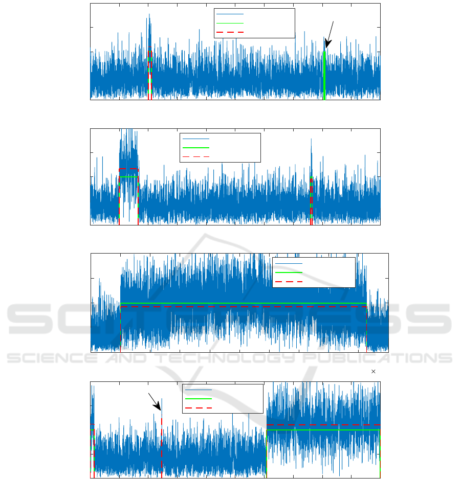
the other 2 measures. Fig. 7 visualizes the estimation

of TOAs and TODs in some parts of the testing signal

for SNR = 6 dB.

6 CONCLUSION

We have presented a deep-learning-based approach

to the detection of radar pulses with various wave-

forms over a wide range of SNRs. The proposed

scheme combines a classical ﬁnd-change-points algo-

rithm with a convolutional neural network for seg-

ment classiﬁcation. Informally speaking, the clas-

siﬁcation net plays a guiding role to facilitate the

ﬁnd-change-points routine. Experiments on simu-

lated data suggest that our method strikingly outper-

forms the Threshold-based Edge Detection (TED) al-

gorithm, especially in low-SNR regimes. Another ad-

vantage of the proposed method is its noise-blindness,

as opposed to TED which heavily relies on a noise

ﬂoor estimation. The shortcoming of our method,

however, is its costly computations, while TED can be

implemented in FPGA for a real-time system. For the

moment, the running time of the algorithm is about

1 µs/sample, which is still far from the real-time tar-

get, 12.8 ns/sample. Future work would, therefore,

focus on reducing the computational cost of the algo-

rithm via a compression of the classiﬁcation net like

what have been done in (Han et al., 2016), as well as

a more efﬁcient implementation of the ﬁnd-change-

points procedure. Another potential direction would

be replacing the ﬁnd-change-points algorithm with a

deep neural network.

REFERENCES

Goodfellow, I., Bengio, Y., and Courville, A. (2016). Deep

Learning. MIT Press.

Han, S., Mao, H., and Dally, W. J. (May 02-04, 2016).

Deep compression: Compressing deep neural net-

works with pruning, trained quantization and huffman

Deep Learning for Radar Pulse Detection

0 1000 2000 3000 4000 5000 6000 7000 8000 9000 10000

Sample

0.5

1.5

Magnitude

Signal envelop

True Pulses

Detected Pulses

Missed

0 1000 2000 3000 4000 5000 6000 7000 8000 9000 10000

Sample

0.5

1.5

Magnitude

Signal envelop

True Pulses

Detected Pulses

0 0.2 0.4 0.6 0.8 1 1.2 1.4 1.6 1.8 2

Sample

0.5

1.5

Magnitude

Signal envelop

True Pulses

Detected Pulses

0 1000 2000 3000 4000 5000 6000 7000 8000 9000 10000

Sample

0.5

1.5

Magnitude

Signal envelop

True Pulses

Detected Pulses

False Alarm

Figure 7: Detection results in different parts of the noisy signal with SNR = 6 dB at bandwidth 20 MHz. For each detected

pulse, the pulse amplitude is estimated by averaging the signal magnitudes in between the estimated TOA and TOD. Misses

and false alarms are marked with arrows.

coding. In Proc. Int. Conf. Learning Representations

(ICLR), pages 1–14, Puerto Rico.

He, K., Zhang, X., Ren, S., and Sun, J. (Jun. 27-30, 2016).

Deep residual learning for image recognition. In Proc.

Conf. Comput. Vis. Pattern Recogn. (CVPR), pages

770–778, Las Vegas, NV, USA.

Iglesias, V., Grajal, J., Yeste-Ojeda, O., Garrido, M.,

anchez, M. A., and L

opez-Vallejo, M. (May 19-23,

2014). Real-time radar pulse parameter extractor. In

Proc. IEEE Radar Conf., pages 1–5.

Ioffe, S. and Szegedy, C. (Jul. 06-11, 2015). Batch nor-

malization: Accelerating deep network training by re-

ducing internal covariate shift. In Proc. Int. Conf.

Machine Learning (ICML), pages 1097–1105, Lille,

France.

Jackson, B., Scargle, J. D., Barnes, D., Arabhi, S., Alt, A.,

Gioumousis, P., Gwin, E., Sangtrakulcharoen, P., Tan,

L., and Tsai, T. T. (2005). An algorithm for optimal

ICPRAM 2019 - 8th International Conference on Pattern Recognition Applications and Methods

partitioning of data on an interval. IEEE Signal Pro-

cess. Lett., 12(2):105 – 108.

Killick, R., Fearnhead, P., and Eckley, I. A. (2012). Optimal

detection of changepoints with linear computational

cost. J. Am. Stat. Assoc., 107(500):1590–1598.

Krizhevsky, A., Sutskever, I., and Hinton, G. E. (Dec. 03-

08, 2012). Imagenet classiﬁcation with deep convo-

lutional neural networks. In Proc. Adv. Neural Inf.

Process. Syst. (NIPS), pages 1097–1105, Lake Tahoe,

NV, USA.

LeCun, Y., Bengio, Y., and Hinton, G. (2015). Deep learn-

ing. Nature, 521:436–444.

Levanon, N. and Mozeson, E. (2004). Radar Signals.

Wiley-Interscience.

Liu, W., Anguelov, D., Erhan, D., Szegedy, C., Reed, S.,

Fu, C.-Y., and Berg, A. C. (Oct. 08-16, 2016). SSD:

Single shot multibox detector. In Proc. Eur. Conf.

Comput. Vis. (ECCV), pages 21–37, Amsterdam, The

Netherlands.

Pace, P. E. (2009). Detecting and Classifying Low Proba-

bility of Intercept Radar. Artech House, 2 edition.

Poisel, R. (2005). EW Target Location Methods. Artech

House.

Redmon, J., Divvala, S., Girshick, R., and Farhadi, A. (Jun.

27-30, 2016). You Only Look Once: Uniﬁed, real-

time object detection. In Proc. Conf. Comput. Vis. Pat-

tern Recogn. (CVPR), pages 779–788, Las Vegas, NV,

USA.

Ren, S., He, K., Girshick, R., and Sun, J. (2017). Faster

R-CNN: Towards real-time object detection with re-

gion proposal networks. IEEE Trans. Pattern Anal.

Machine Intell., 39(6):1137–1149.

Richards, M. A. (2014). Fundamental of Radar Signal Pro-

cessing. McGraw-Hill Education, 2 edition.

Szegedy, C., Liu, W., Jia, Y., Sermanet, P., Reed, S.,

Anguelov, D., Erhan, D., Vanhoucke, V., and Rabi-

novich, A. (Jun. 07-12, 2015). Going deeper with

convolutions. In Proc. Conf. Comput. Vis. Pattern

Recogn. (CVPR), pages 1–9, Boston, MA, USA.

Torrieri, D. J. (1974). Arrival time estimation by adaptive

thresholding. IEEE Trans. Aerospace Electro. Sys-

tems, AES-10(2):178–184.

Torrieri, D. J. (1984). Statistical theory of passive location

systems. IEEE Trans. Aerospace Electro. Systems,

AES-20(2):183–198.

Deep Learning for Radar Pulse Detection