
Deep Learning for Pulse Repetition Interval Classification
Ha P. K. Nguyen, Ha Q. Nguyen and Dat T. Ngo
Viettel Research and Development Institute, Hoa Lac High-tech Park, Hanoi, Vietnam
Keywords:
Pulse Repetition Intervals, PRI Modulation Classification, Convolutional Neural Network, Deep Learning.
Abstract:
Pulse Repetition Intervals (PRI)—the distances between consecutive times of arrival of radar pulses—is an
important characteristic of the radar emitting source. The recognition of various PRI modulation types is
therefore a key task of an Electronic Support Measure (ESM) system for accurate identification of threat
emitters. This problem is challenging due to the missing and spurious pulses. In this paper, we introduce
a deep-learning-based method for the classification of 7 popular PRI modulation types. In this approach, a
convolutional neural network (CNN) is proposed as the classifier. Our method works well with raw input
PRI sequences and, thus, gets rid of all preprocessing steps such as noise mitigation, feature extraction, and
threshold setting, as required in previous approaches. Extensive simulations demonstrate that the proposed
scheme outperforms existing methods by a significant margin over a variety of PRI parameters, especially in
severely noisy conditions.
1 INTRODUCTION
An Electronic Support Measures (ESM) system cap-
tures radar signals from multiple sources and identi-
fies the radars based on several characteristics of the
received signals. One of the most important features
of a radar signal is the sequence of pulse repetition
intervals (PRI) that consists of distances between the
times of arrival (TOAs) of consecutive radar pulses.
In modern radar technology, various types of com-
plicated PRI modulation are used rather than just a
simple constant pattern. Therefore, the recognition of
PRI modulations will greatly help identify the emit-
ting sources. This is, however, far from a trivial prob-
lem due to the unavoidable miss-detections and false
alarms of the TOAs, which might result in very noisy
PRI sequences. In addition, the diversity of parame-
ters in each type of PRI modulation makes the recog-
nition task much more challenging.
To solve the PRI modulation classification is-
sue, extensive research has been conducted. Existing
methods can generally be divided into 3 categories:
statistics-based, decision-tree-based, and learning-
based. In the classical statistics-based methods (Mar-
dia, 1989; Milojevic and Popovic, 1992), histogram
techniques are used to recognize PRI modulation
types. Since these methods are simple, they work only
with a limited number of PRI modulation types and
their performances are drastically degraded in noisy
situations. Decision-tree based methods (Kauppi and
Martikainen, 2007; Hu and Liu, 2010; Song et al.,
2010) usually consist of three steps: first, a noise mit-
igation technique is applied to compensate the impact
of missing and spurious pulses on the PRI sequence;
second, discriminative features are extracted from the
denoised PRI sequence; and, finally, a decision-tree is
carried out to differentiate PRI modulation types. The
main shortcoming of decision-tree-based approaches
is the requirement of heavily-handcrafted thresholds,
which are not only time-consuming but also very sen-
sitive to the level of noise and the change of PRI pa-
rameters. Existing learning-based methods for PRI
modulation classification often rely on shallow neu-
ral networks. Noone proposed in (Noone, 1999) a
neural-network classifier with a single hidden layer
that is trained on a set of the second differences of
the TOAs. More recently, Liu and Zhang introduced
in (Liu and Zhang, 2017) a feed-forward neural net-
work consisting of an input layer with 3 features de-
rived from (Noone, 1999) and a single hidden layer
of only 8 neurons. This method can only classify 4
types of PRI modulations. It is noteworthy that all
the aforementioned learning-based methods require a
careful design of features and a feature extraction pro-
cess before the neural network can be applied. This
drawback prevents these methods from quick adapta-
tion to changes in the PRI modulations.
Recently, deep learning (LeCun et al., 2015;
Goodfellow et al., 2016) has emerged as a power-
ful tool for many classification tasks. In this paper,
Nguyen, H., Nguyen, H. and Ngo, D.
Deep Learning for Pulse Repetition Interval Classification.
DOI: 10.5220/0007253203130319
In Proceedings of the 8th International Conference on Pattern Recognition Applications and Methods (ICPRAM 2019), pages 313-319
ISBN: 978-989-758-351-3
Copyright
c
2019 by SCITEPRESS – Science and Technology Publications, Lda. All rights reserved
313
we introduce a novel deep-learning-based scheme in
which a deep Convolutional Neural Network (CNN)
is trained to classify 7 types of PRI modulations.
To the best of our knowledge, we are the first to
adopt a deep learning approach to solve this prob-
lem. The main advantage of the proposed method
is that the CNN takes raw PRI sequences as input
and, therefore, bypasses the feature extraction proce-
dures as in previous approaches. Furthermore, as will
be demonstrated in simulations, our approach is very
noise-robust and effective for classifying PRI modu-
lations compared to existing methods. In particular,
for a wide range of missing and spurious pulse frac-
tions, the proposed method noticeably outperforms
the other competitors with an accuracy gap of at least
2%. This gap even increases quickly with the noise
level.
The rest of this paper is organized as follows: Sec-
tion 2 presents some preliminaries about PRI mod-
ulations; Section 3 describes the architecture of the
CNN; Section 4 evaluates the performance of the pro-
posed method on simulated data against state-of-the-
art classifiers; and, finally, Section 5 concludes the
paper.
2 PRI MODULATIONS
An ESM system receives radar signals and estimates
the parameters associated with each of the detected
pulses. Given a sequence of TOAs of the radar signal
{t[n]}
N
n=0
, where t[n] is the estimated arrival time of
the nth radar pulse and N is the number of detected
pulses, the PRI sequence is defined as
p[n] = t[n +1] − t[n], n = 0,... ,N − 1. (1)
The pattern of a PRI sequence is dictated by a specific
PRI modulation type. In this paper, we consider the
following 7 PRI modulation types that are frequently
used in modern radar systems:
1. Constant (CST): the simplest PRI modulation in
which the pulses are equally spaced.
2. Sliding Up (SLU): the PRIs periodically linearly
increase with respect to some slope.
3. Sliding Down (SLD): the PRIs periodically lin-
early decrease with respect to some slope.
4. Jittered (JIT): the PRIs are randomized according
to a Gaussian distribution.
5. Staggered (STG): the PRIs periodically jump
through a fixed number of levels.
6. Dwell & Switch (DS): piecewise-constant PRIs,
where each piece is called a burst.
0 0.05 0.1
Time (sec)
700
750
800
850
900
PRI (usec)
(a) CST
0 0.05 0.1
Time (sec)
300
400
500
600
700
800
900
PRI (usec)
(b) SLU
0 0.05 0.1
Time (sec)
300
400
500
600
700
800
900
PRI (usec)
(c) SLD
0 0.05 0.1
Time (sec)
700
750
800
850
900
PRI (usec)
(d) JIT
0 0.05 0.1
Time (sec)
700
750
800
850
900
PRI (usec)
(e) STG
0 0.05 0.1
Time (sec)
700
750
800
850
900
PRI (usec)
(f) DS
0 0.05 0.1
Time (sec)
700
750
800
850
900
PRI (usec)
(g) WOB
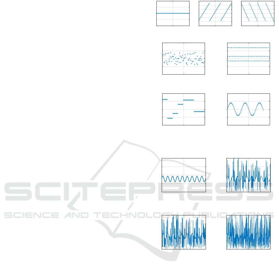
Figure 1: Ideal examples of the 7 PRI modulations.
0 0.05 0.1
Time (sec)
0
1000
2000
3000
4000
PRI (usec)
(a) ideal
0 0.05 0.1
Time (sec)
0
1000
2000
3000
4000
PRI (usec)
(b) 5%
0 0.05 0.1
Time (sec)
0
1000
2000
3000
4000
PRI (usec)
(c) 10%
0 0.05 0.1
Time (sec)
0
1000
2000
3000
4000
PRI (usec)
(d) 30%
Figure 2: A Wobulated PRI sequence with different frac-
tions of missing and spurious pulses. Each subplot from
(b) to (d) is captioned with the rate of missing and spurious
pulses.
7. Wobulated (WOB): sinusoidal PRIs.
Fig. 1 illustrates ideal examples of these PRI mod-
ulations. In practice, however, PRIs are subject to per-
turbations, miss-detections (missing pulses) and false
alarms (spurious pulses) due to the imperfection of
the TOA estimation process. The combined effect
of these errors may significantly distort the original
form of a PRI sequence, as showed in Fig. 2, posing a
great challenge for the classification task. A common
method for suppressing the speckle noise on PRI se-
quences is to apply median filters as a preprocessing
step. However, the choice of the filter length, which
ICPRAM 2019 - 8th International Conference on Pattern Recognition Applications and Methods
314

is critical, is very sensitive to the noise level. Fur-
thermore, the median filtering might destroy the pat-
tern of the PRIs, making the classification even harder
in some cases. Also, note that existing classification
methods rely on handcrafted features and/or thresh-
olds are that are not robust to a wide range of noise
imposed on PRI sequences. The above shortcomings
can be overcome with a deep Convolutional Neural
Network (CNN) as will be described next.
3 CNN ARCHITECTURE
We propose in this section a CNN, whose architecture
is depicted in Fig. 3, for the PRI classification. As op-
posed to the previous neural-network schemes, the in-
put to the proposed CNN is the raw PRI sequence of
fixed size 1 × 1000, supposedly obtained from a TOA
estimation algorithm. That is, both the denoising and
the feature extraction are handled by the network it-
self. This is done via a concatenation of 8 convolution
layers and 2 fully connected (dense) layers. Roughly
speaking, the convolution layers play the role of a fea-
ture extraction that is robust to noise, while the dense
layers take care of the classification based on the out-
put of the final convolution layer. The whole network
is trained end-to-end on a dataset of PRI sequences
labeled with ground-truth modulation types indexed
from 0 to 6. Note that before feeding a PRI sequence
p[n] to the network, we normalize it as
p
norm
[n] =
p[n]
max
i
p[i]
, ∀n. (2)
Following the design philosophy of the VGG-
net (Simonyan and Zisserman, 2015), all filters used
in the 8 convolution layers are of fixed size 1 × 3,
resulting in a receptive field of 8 × 2 + 1 = 17 sam-
ples. The number of filters is decreased from 32 to 4
along the convolution layers. Note that, in each con-
volution layer, a batch normalization is used to com-
bat the internal covariate shift as suggested in (Ioffe
and Szegedy, 2015). Moreover, the Rectified Linear
Unit (ReLU) is used as the activation function for all
convolution layers. The result of the final convolu-
tion layer is 4 feature maps, each of size 1 × 1000,
which are then flattened into a single feature vector
of length 4000. This vector is fully connected to a
layer of 256 neurons with ReLU activation. To pre-
vent over-fitting, a dropout layer (Srivastava et al.,
2014) with dropping ratio of 0.7 is inserted in be-
tween these layers. Finally, the output of the Dense-
256 layer is transformed to a score vector of length
7 via the last fully connected layer with the softmax
activation function. The score vector can be thought
of as a probability distribution of the 7 classes.
The network weights are trained by minimizing
a loss function defined as the cross-entropy between
the output vector of the network and the one-hot vec-
tor associated with the ground-truth label of the input
PRI sequence. This optimization procedure can be re-
alized by a stochastic gradient descent algorithm. In
the testing phase, the class of an input PRI sequence
is simply determined by taking the index of the output
vector that yields the maximum score.
4 PERFORMANCE EVALUATION
In order to evaluate the performance of our CNN-
based PRI classification, a set of 140,000 randomly
generated PRI sequences (20,000 for each modulation
type) was used for training and another set of 35,000
(5,000 for each class) was used for testing. Both train-
ing and testing data were generated randomly accord-
ing to a variety of parameters given in Table 1. It
should be noted that the training set and the testing set
are separated and different from each other. There-
fore, the testing set can be fairly used to verify the
accuracy and generalization of the proposed model.
The data generation was performed in Matlab, while
the training was implemented in Python with Keras li-
brary and TensorFlow backend, running on an Nvidia
Tesla P100 GPU. The final CNN model was obtained
after being trained for 100 epochs with Adam opti-
mizer and with a learning rate of 10
−4
.
We compare CNN with 3 state-of-the-art competi-
tors including both decision-tree-based and learning-
based methods as follows:
• The proposed scheme in (Song et al., 2010): This
method is able to classify only 5 PRI modula-
tion types (DS, SLD, SLU, JIT, and WOB) by ap-
plying a decision tree on features extracted from
the symbolizations of PRI and differential PRI
sequences. Hence, we refer to this method as
Symbolization-based Decision Tree (SDT). The
thresholds used in this algorithm were carefully
chosen to optimize the classification accuracy.
• The proposed scheme in (Noone, 1999), which
we call Transform-based Neural Network (TNN):
This learning-based method uses the second dif-
ferences of TOAs feature as the input of a feed-
forward neural-network.
• The proposed scheme in (Liu and Zhang, 2017):
This method uses a feed forward neural network
consisting of an input layer with 3 extracted fea-
tures based on the second differences of TOAs to
classify 4 PRI modulation types (WOB, JIT, DS,
and Sliding). It should be noted that in that pa-
Deep Learning for Pulse Repetition Interval Classification
315
Figure 3: Architecture of the proposed CNN for PRI classification.
Table 1: PRI parameters used in simulations. Each PRI
sequence is generated by a combination of parameters ran-
domly selected from the given ranges.
Type Parameters
All
Number of TOAs = 1001
PRI pertubation = ±(0.5 ÷ 2.0)µs
Rate of Missing pulses = (0 ÷ 30)%
Rate of Spurious pulses = (0 ÷ 30)%
CST PRI value = (50 ÷ 4000)µs
STG
PRI value = (50 ÷ 4000)µs
Number of PRI levels = (2 ÷ 10)
JIT
PRI value = (50 ÷ 4000)µs
PRI deviation = (5 ÷ 20)% of PRI value
DS
PRI value = (50 ÷ 4000)µs
Number of bursts = (2 ÷ 10)
Burst length = (30 ÷ 120) pulses
Sliding
PRI
max
/PRI
min
ratio = (2 ÷ 6)
PRI
max
∈
{
200,600,1000, 1500,2000, 4000
}
Number of slides = (2 ÷ 10)
WOB
PRI mean value = (50 ÷ 2000)µs
PRI
max
/PRI
mean
ratio = (1.02 ÷ 1.5)
Number of periods = (2 ÷ 10)
per, the authors combined two PRI modulations,
SLU and SLD, into a single type called Slid-
ing (SL). We name this scheme Improved Feed-
forward Neural Network (IFNN).
Since TNN and IFNN are also learning-based, for
a fair comparison, they were trained on the same train-
ing dataset of CNN. The training of these two net-
works was done in Matlab with Neural Network Tool-
box. After training all the models, we used the same
testing dataset to verify the PRI classification accu-
racy of CNN, TNN, IFNN, and SDT. The comparison
of the 4 methods was performed on a mixed dataset
of all noise levels, as well as on several datasets of
specific noise levels.
4.1 Overall Accuracy
Figs. 4, 5, and 6 show the training and testing confu-
sion matrices of CNN, TNN, and IFNN, respectively.
Since SDT is a decision-based method without any
training, we only report the confusion matrix of the
testing dataset for this scheme in Fig. 7. It can be seen
from Fig. 4 that the proposed CNN achieves a classifi-
cation accuracy of 99.40% and 98.42% on the training
dataset and testing dataset, respectively. It means that
the recognition correctness of CNN is 24.42% higher
than that of a typical decision-tree-based scheme,
SDT. CNN also yields a superior performance com-
pared to TNN, which only reaches a classification ac-
curacy of 63.35% on the testing dataset. Additionally,
comparing to a recent learning-based method, IFNN,
CNN also improves the classification performance by
about 2%. It is worth noting that our proposed scheme
outperforms SDT and IFNN, although it should clas-
sify for many more PRI modulation classes. More-
over, by using only the raw noisy PRI sequences as
input, our method can get rid of the threshold setting
process of SDT and the preprocessing steps, such as
noise compensation and feature extraction, of TNN
and IFNN.
4.2 Accuracy with Varying Noise
In this subsection, we further investigate the effect of
missing pulse rate and spurious pulse rate on the clas-
sification performance. We tested our CNN method
against the other competitors under various noisy con-
ditions by using different datasets with varying ranges
of missing pulse rate and spurious pulse rate as fol-
lows:
• Dataset 1: Rates of missing and spurious pulses
are randomly varied from 0% to 5%;
• Dataset 2: Rates of missing and spurious pulses
are randomly varied from 5% to 10%;
• Dataset 3: Rates of missing and spurious pulses
are randomly varied from 10% to 15%;
• Dataset 4: Rates of missing and spurious pulses
are randomly varied from 15% to 20%;
• Dataset 5: Rates of missing and spurious pulses
are randomly varied from 20% to 25%;
ICPRAM 2019 - 8th International Conference on Pattern Recognition Applications and Methods
316
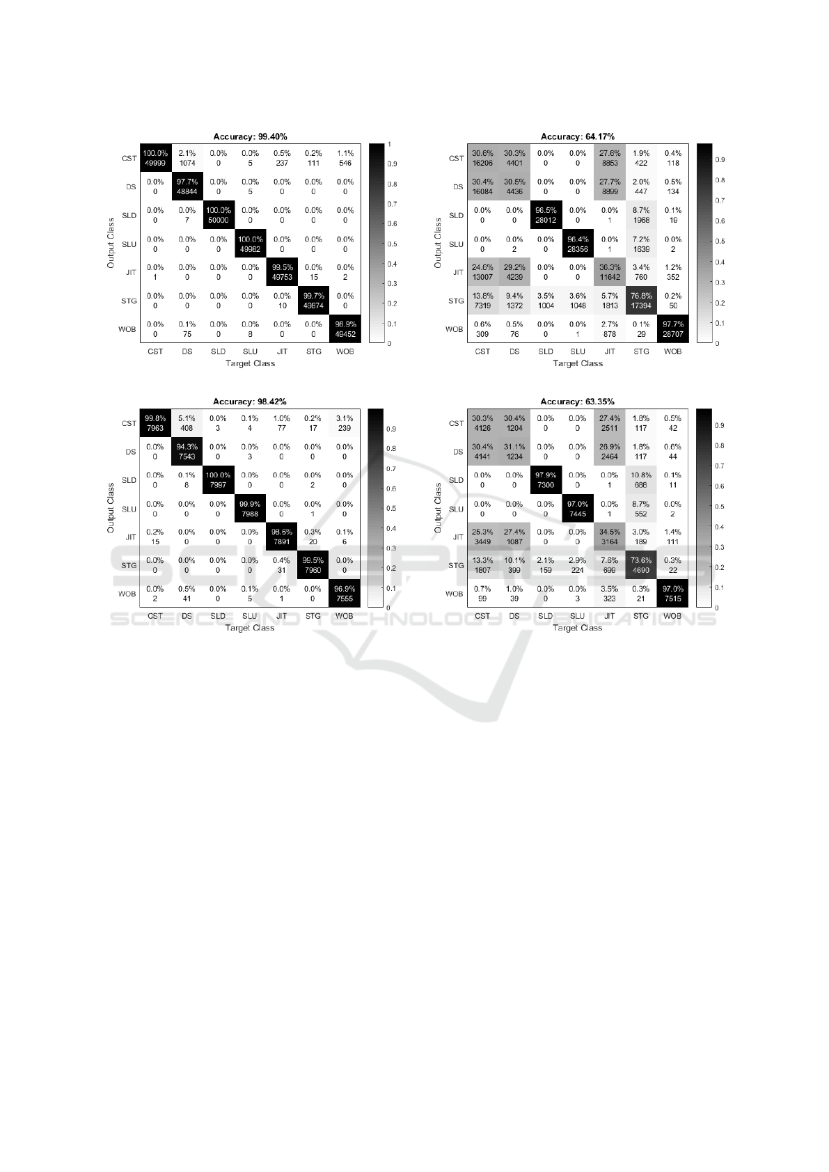
(a) Training
(b) Testing
Figure 4: Confusion matrices of CNN on the whole testing
dataset with the rates of missing and spurious pulses ranging
from 0% to 30%.
• Dataset 6: Rates of missing and spurious pulses
are randomly varied from 25% to 30%.
Each of the above dataset contains 3000 samples for
each PRI modulation type and is generated randomly
with parameters presented in Table 1. Fig. 8 com-
pares the classification accuracies of the 4 methods
with varying ranges of missing and spurious pulse
rate. It can be observed that TNN achieves the worst
performance. The reason is that the second differ-
ence of PRI sequence is not adequate to discrimi-
nate many complex PRI modulation types. This fea-
ture is also very sensitive with missing and spurious
pulses. In less noisy conditions, SDT performs quite
well with an accuracy greater than 90%. However, its
quality is seriously degraded when the missing and
spurious pulse rates increase. Specifically, the accu-
racy of SDT is reduced by more than 40% when the
fractions of missing and spurious pulse exceed 20%.
(a) Training
(b) Testing
Figure 5: Confusion matrices of TNN on the whole testing
dataset with the rates of missing and spurious pulses ranging
from 0% to 30%.
This observation proves that the fixed thresholding
of decision-tree-based methods is very vulnerable to
noise and, thus, fails to classify the PRI modulations
over a large range of miss-detections and false alarms.
It is remarkable that CNN and IFNN significantly
outperform SDT and TNN. When the missing and
spurious pulse rates are less than 20%, the classifi-
cation accuracy of CNN and IFNN are 99.1% and
97.5% on average, respectively. Nevertheless, the
performance gap between CNN and IFNN increases
considerably with the rates of missing and spurious
pulses. For instance, CNN attains an improvement of
6% compared to IFNN when the missing and spuri-
ous pulse rates are in the range from 25% to 30%.
Again, we recall that CNN outperforms IFNN with
many more classified PRI modulation types (7 of
CNN against 4 of IFNN).
Deep Learning for Pulse Repetition Interval Classification
317
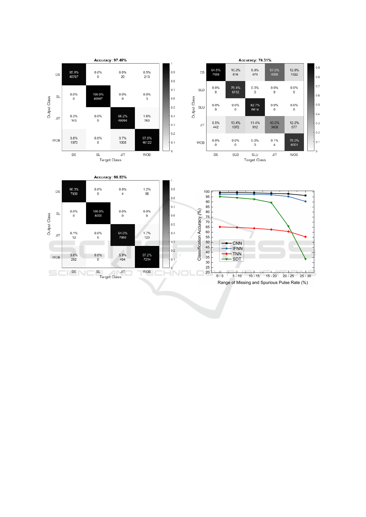
(a) Training
(b) Testing
Figure 6: Confusion matrices of IFNN on the whole testing
dataset with the rates of missing and spurious pulses ranging
from 0% to 30%.
From the above analysis, we can conclude that our
CNN classifier is able to recognize different PRI mod-
ulation types with high accuracy and is resilient to
heavily missing and spurious pulses.
5 CONCLUSION
In this paper, we have proposed a deep-learning-
based method to solve the PRI modulation classifi-
cation for the first time. We have trained a convo-
lution neural network that can efficiently recognize
7 PRI modulation types. The major advantage of
the proposed method is twofold. First, the input of
our classifier is raw PRI sequences; thus, it can by-
pass the noise filtering and the tedious calibration of
many thresholds in decision-tree-based methods, as
well as the feature extraction in previous learning-
Figure 7: Confusion matrices of SDT on the whole testing
dataset with the rates of missing and spurious pulses ranging
from 0% to 30%. Training is not needed for this method.
Figure 8: Classification accuracies of the 4 different meth-
ods are plotted against the range of missing and spurious
rate.
based approaches. Second, in severely noisy environ-
ments with high missing and spurious pulse rates, our
scheme still achieves an impressive classification ac-
curacy, in contrast to other methods. The simulation
results have demonstrated that our proposed method
strikingly surpasses the state-of-the-art PRI classifiers
on a wide range of simulation parameters. For fu-
ture research, it is worth investigating deep neural
networks for estimating the parameters associated to
each type of PRI modulation after the classification.
REFERENCES
Goodfellow, I., Bengio, Y., and Courville, A. (2016). Deep
Learning. MIT Press.
Hu, G. and Liu, Y. (2010). An efficient method of pulse rep-
etition interval modulation recognition. In Proc. IEEE
ICPRAM 2019 - 8th International Conference on Pattern Recognition Applications and Methods
318

Int. Conf. Commun. Mobile Comput., pages 287–295,
Shenzhen, China.
Ioffe, S. and Szegedy, C. (Jul. 06-11, 2015). Batch nor-
malization: Accelerating deep network training by re-
ducing internal covariate shift. In Proc. Int. Conf.
Machine Learning (ICML), pages 1097–1105, Lille,
France.
Kauppi, J.-P. and Martikainen, K. S. (2007). An efficient
set of features for pulse repetition interval modulation
recognition. In Proc. IET Int. Conf. Radar Syst., pages
1–5, Edinburgh, UK.
LeCun, Y., Bengio, Y., and Hinton, G. (2015). Deep learn-
ing. Nature, 521:436–444.
Liu, Y. and Zhang, Q. (2017). An improved algorithm for
PRI modulation recognition. In Proc. IEEE Int. Conf.
Signal Process. Commun. Comput., pages 1–5, Xia-
men, China.
Mardia, H. K. (1989). New techniques for the deinterleav-
ing of repetitive sequences. IEE Proc. F Commun.
Radar & Signal Process., 136(4):149–154.
Milojevic, D. J. and Popovic, B. M. (1992). Improved algo-
rithm for the deinterleaving of radar pulses. IEE Proc.
F Commun. Radar & Signal Process., 139(1):98–104.
Noone, G. P. (1999). A neural approach to automatic pulse
repetition interval modulation recognition. In Proc.
IEEE Information, Decision and Control (IDC), pages
213–218, Phoenix, AZ, USA.
Simonyan, K. and Zisserman, A. (2015). Very deep con-
volutional networks for large-scale image recognition.
In Proc. Int. Conf. Learning Representations (ICLR),
pages 1–14, San Diego, USA.
Song, K. H., Lee, D. W., Han, J. W., and Park, B. K. (2010).
Pulse repetition interval modulation recognition using
symbolization. In Proc. IEEE Int. Conf. Digit. Im-
age Comput.: Techniques and Applications (DICTA),
pages 540–545, Sydney, NSW, Australia.
Srivastava, N., Hinton, G., Krizhevsky, A., Sutskever, I.,
and Salakhutdinov, R. (2014). Dropout: A simple
way to prevent neural networks from overfitting. J.
Machine Learning Research, 15(1):1929–1958.
Deep Learning for Pulse Repetition Interval Classification
319
