Multiclass Tissue Classiﬁcation of Whole-Slide Histological Images using

Convolutional Neural Networks

Rune Wetteland

, Kjersti Engan

, Trygve Eftestøl

, Vebjørn Kvikstad

and Emilius A. M. Janssen

2,3

Department of Electrical Engineering and Computer Science, University of Stavanger, Norway

Department of Pathology, Stavanger University Hospital, Norway

Department of Mathematics and Natural Sciences, University of Stavanger, Norway

Keywords:

Histological Whole-Slide Images, Autoencoder, Deep Learning, Semi-supervised Learning, ROI Extraction.

Abstract:

Globally there has been an enormous increase in bladder cancer incidents the past decades. Correct prognosis

of recurrence and progression is essential to avoid under- or over-treatment of the patient, as well as unnec-

essary suffering and cost. To diagnose the cancer grade and stage, pathologists study the histological images.

However, this is a time-consuming process and reproducibility among pathologists is low. A ﬁrst stage for an

automated diagnosis system can be to identify the diagnostical relevant areas in the histological whole-slide

images (WSI), segmenting cell tissue from damaged areas, blood, background, etc. In this work, a method

for automatic classiﬁcation of urothelial carcinoma into six different classes is proposed. The method is based

on convolutional neural networks (CNN), ﬁrstly trained unsupervised using unlabelled images by utilising an

autoencoder (AE). A smaller set of labelled images are used to train the ﬁnal fully-connected layers from the

low dimensional latent vector of the AE, providing an output as a probability score for each of the six classes,

suitable for automatically deﬁning regions of interests in WSI. For evaluation, each tile is classiﬁed as the class

with the highest probability score. The model achieved an average F1-score of 93.4% over all six classes.

1 INTRODUCTION

Globally, bladder cancer resulted in 123,400 deaths in

1990, and in 2010 this number was 170,700 which is

an increase of 38,3% taking population growth into

consideration (Lozano et al., 2012). The majority

of bladder cancer incidents are urothelial carcinoma

with a representation as high as 90% in some regions

(Eble et al., 2004). For patients diagnosed with blad-

der cancer, 50-70% will experience one or more re-

currences, and 10-30% will have disease progression

to a higher stage (Mangrud, 2014). Patient treatment,

follow-up and calculating the risk of recurrence and

disease progression depend primarily on the histolog-

ical grade and stage of cancer. Correct prognosis of

recurrence and progression is essential to avoid under-

or over-treatment of the patient, as well as unneces-

sary suffering and cost.

With the introduction of digital pathology, some

computer-aided tools to assist pathologists have been

introduced, but still the assessment of histopatholog-

ical images to diagnose, grade and stage cancer is

mainly done manually. This is a time-consuming

process and reproducibility among pathologists is in

some cases low, for example within the prognostic

classiﬁcation of urinary bladder cancer. Automatic

extraction of the relevant areas in large whole-slide

images (WSI) would be an important ﬁrst step where

the results could be used in automated diagnostic and

prognostic classiﬁcation tools.

During the biopsy, parts of the tissue get both

physical- and heating-damage, and thus can not be

used as relevant diagnostic information. The WSI

also contains stroma- and muscle-tissue as well as ar-

eas of blood. In this paper we consider the task of

automatic classiﬁcation of tiles in WSI into the six

different classes; urothelium, stroma, damaged tissue,

muscle, blood and background. Examples from each

class are shown in Figure 1. The system uses the au-

tomatic classiﬁcation tool to produce heat maps from

the model’s output. Such heat maps can provide use-

ful information to help the pathologist to focus on the

diagnostic important part of the large WSI during vi-

sual inspection. In addition, the heat maps are also

suitable as input for automatic region of interest (ROI)

extraction of relevant areas in the WSI, which can fur-

ther be used in automated diagnostic and prognostic

classiﬁcation tools.

320

Wetteland, R., Engan, K., Eftestøl, T., Kvikstad, V. and Janssen, E.

Multiclass Tissue Classiﬁcation of Whole-Slide Histological Images using Convolutional Neural Networks.

DOI: 10.5220/0007253603200327

In Proceedings of the 8th International Conference on Pattern Recognition Applications and Methods (ICPRAM 2019), pages 320-327

ISBN: 978-989-758-351-3

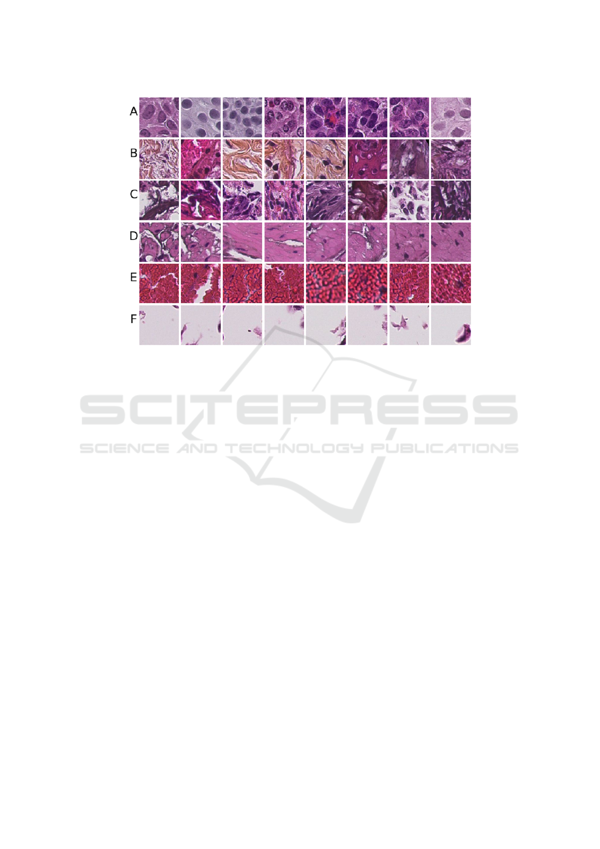
Figure 1: Example tiles from each class. A) Urothelium, B) Stroma, C) Damaged tissue, D) Muscle tissue, E) Blood, and F)

Background.

1.1 Previous Work

In recent literature, some methods for automatic tis-

sue classiﬁcation have been suggested. However,

most previous works have focused on classifying only

two classes, a binary problem set to differentiate be-

tween cancer-patches and non-cancer patches.

Recent literature shows good results for binary tis-

sue classiﬁcation using convolutional neural networks

(CNN). Wang et al. (2016) won both competitions of

the Camelyon16 grand challenge for automated de-

tection of metastatic breast cancer in WSI. As part

of their model, GoogLeNet was utilised to do patch

classiﬁcation. The model was trained to discriminate

between positive and negative patches and achieved

an accuracy of 98.4%.

Some attempts of multiclass tissue classiﬁcation

can be found in recent years. Araujo et al. classiﬁed

patches of breast cancer into four classes using con-

volutional neural networks (Ara

ujo et al., 2017). The

best patch-wise accuracy for four classes was 66.7%.

When the task was simpliﬁed as a two-classes prob-

lem, non-carcinoma vs carcinoma, the accuracy was

improved to 77.6%. The work of Kather et al. (2016)

uses a combination of several hand-crafted feature

methods to classify different types of tissue in col-

orectal cancer, performing tests on both a two-class

and eight-class problem. They achieved the best re-

sult on the two-class problem with a tumour-stroma

separation accuracy of 98.6%, while the multiclass

problem achieved an accuracy of 87.4%.

To the author’s knowledge, there are no published

results on multiclass classiﬁcation on WSI of bladder

cancer.

Some few and recent work on ROI detection can

be found. ROI detection has been done by multi-scale

real-time coarse-to-ﬁne topology preserving segmen-

tation (CTFTPS) by utilising superpixel clustering

technique (Li and Huang, 2015; Yao et al., 2015).

A RAPID (Regular and Adaptive Prediction-Induced

Detection) segmentation method for ROI detection in

large WSI is presented by Sulimowicz and Ahmad

(2017) while using the multi-scale CTFTPS technique

as a baseline. An SVM was utilised to classify the

detected regions as ROI vs non-ROI. For this task,

the classiﬁer achieved an F1-score of 89.8% for the

RAPID method, and 91.2% for the optimised multi-

scale CTFTPS method.

Deep CNN has shown to provide state of the

art results in many computer vision tasks in recent

years (LeCun et al., 2015) and has also found its way

into medical image assessment tasks. In this work,

a method for automatic classiﬁcation of WSI from

urothelial carcinoma into six different classes is pro-

posed. The method is based on CNN, ﬁrstly trained

unsupervised, using large unlabelled image sets by

utilising an autoencoder (AE). A set of labelled im-

ages are used to train the ﬁnal fully-connected layers

from the low dimensional latent vector of the AE, pro-

viding an output as a probability score for each of the

Multiclass Tissue Classiﬁcation of Whole-Slide Histological Images using Convolutional Neural Networks

321

nostra, per inceptos himenaeos. Proin rutrum risus id sodales laoreet. Aenean tincidunt porta est. Ut suscipit, ligula tincidunt lacinia interdum, urna sapien rutrum orci, vitae consequat ex

elit at ipsum. Cras et arcu at justo ultrices tincidunt. Sed maximus libero at neque lobortis ultricies. Suspendisse quis quam nibh. Quisque rhoncus fringilla facilisis.

Lorem ipsum dolor sit amet, consectetur adipiscing elit. Donec diam leo, consectetur ac feugiat eget, laoreet id eros. Phasellus lectus mi, scelerisque ac finibus a, dictum id arcu. Nunc

vehicula ante erat, id faucibus sapien placerat id. Vivamus ultricies diam non magna iaculis gravida. Cras lacinia scelerisque lacus, non consequat nisl hendrerit nec. Aliquam viverra, nisl

ut pretium egestas, metus dolor feugiat purus, in malesuada sem quam id neque. Donec eleifend vestibulum enim at auctor. Class aptent taciti sociosqu ad litora torquent per conubia

nostra, per inceptos himenaeos. Proin rutrum risus id sodales laoreet. Aenean tincidunt porta est. Ut suscipit, ligula tincidunt lacinia interdum, urna sapien rutrum orci, vitae consequat ex

elit at ipsum. Cras et arcu at justo ultrices tincidunt. Sed maximus libero at neque lobortis ultricies. Suspendisse quis quam nibh. Quisque rhoncus fringilla facilisis.

Decoder

Classifier

128x128x8

64x64x8

Reconstructed tile

(128x128x3)

32x32x8

4096

2048

8192

Classifier

6) Background

1 %6

5) Blood

4) Muscle tissue

3)Damagedtissue

2) Stroma

1) Urothelium

1 %

2 %4

6 %3

21 %

69 %1

Probability

output

256

Encoder

128x128x8

64x64x8

Input tile

(128x128x3)

4096

2048

32x32x8

Latent

vector

1024

Unlabelled dataset

Max PoolingConvolution Dropout Fully-connected Deconvolution Unpooling

Whole-Slide Images

Labelled dataset

512

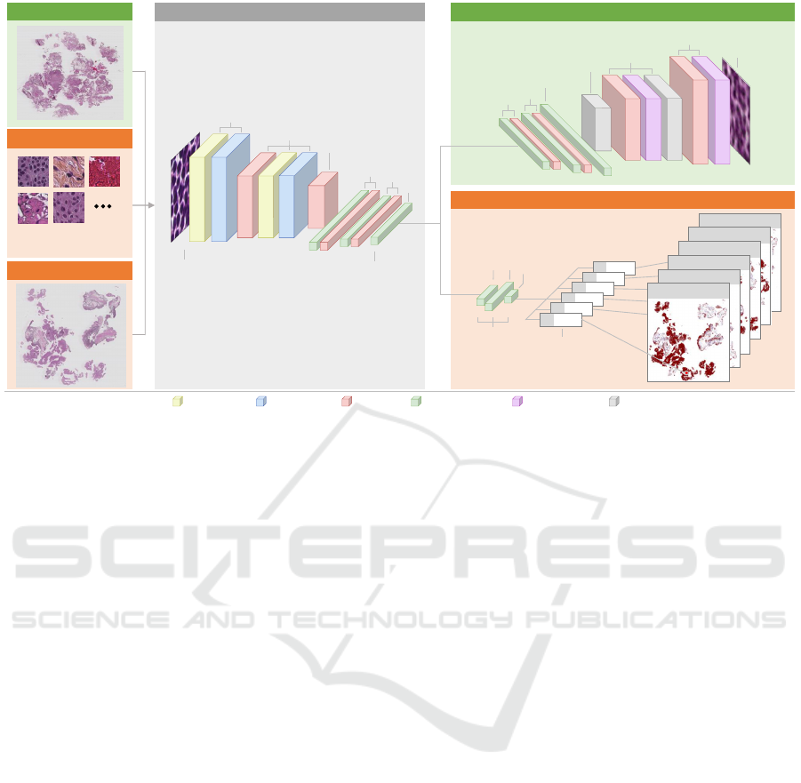
Figure 2: Overview of the CNN-model. First, the unlabelled dataset is used to train the encoder-decoder model. Then the

labelled dataset is used to train the encoder-classiﬁer model. Finally, the trained encoder-classiﬁer model are used to classify

new WSI into probability maps. These probability maps are further postprocessed to produce the heat maps.

six classes, suitable for automatically deﬁning ROI in

WSI. A visualisation of the system is depicted in Fig-

ure 2.

The novelty of the work lies both in the speciﬁc

application of urinary bladder WSI and in the method

development, more speciﬁcally in a combination of

using CNN, learned in a semi-supervised way, for the

application of automatic region of interest extraction

in WSI by multiclass tissue classiﬁcation, tested on

urinary bladder cancer.

2 DATA MATERIAL

The data material used in this paper consists of

histopathological images from patients with primary

bladder cancer, collected in the period 2002-2011 at

the University Hospital of Stavanger in Norway. The

biopsies are formalin ﬁxed and parafﬁn embedded, 4

µm slides are cut and stained with Hematoxylin Eosin

Saffron (HES). All slides are diagnosed and graded

according to WHO73 and WHO04, cancer stage (Tis,

Ta or T1) and follow-up data on recurrence and dis-

ease progression are recorded.

The slides are then scanned using a Leica SCN400

histological slide scanner to produce a digital histo-

logical image. The images are in Leicas data format

called SCN and to be able to process these images

the Vips library (Martinez and Cupitt, 2005) has been

used, which is specially designed for image

processing of large images.

3 PROPOSED METHOD

An overview of the proposed method can be seen in

Figure 2. The different parts will be explained in this

section.

3.1 Preprocessing

Each WSI is sliced into smaller non-overlapping tiles

of size 128x128 pixels, extracted at 400x magniﬁca-

tion level. The background takes up as much as 70-

80% of the WSI and is detected and discarded auto-

matically by computing the histogram of the tile and

setting a ﬁxed threshold value. This removes tiles

consisting of grey background, however, if the back-

ground tile contains small parts of debris, tissue or

similar it is not discarded. Examples of tiles belong-

ing to this class are illustrated in Figure 1-F.

The histological images are split into three

datasets. First, an unlabelled dataset is created in

the manner explained above where the extracted tiles

have no label associated with it. In total 48 WSI all

from different patients were preprocessed resulting in

7,130,527 unlabelled tiles after the pure background

tiles are excluded. This set, called train-ae, is utilised

ICPRAM 2019 - 8th International Conference on Pattern Recognition Applications and Methods

322

as training data for the AE-model.

Secondly, a labelled training dataset is created. A

pathologist has manually annotated carefully selected

regions in the WSI. The tiles in the regions are pre-

processed by evaluating the histogram to be sure not

to include background or boundaries and given a la-

bel corresponding to its class. The number of patients

and tiles produced are listed as train-set1 in Table 1.

Lastly, a labelled test set is created to assess the

performance of the classiﬁer. The set is created in

the same manner as the labelled training set, but

on separate WSI which has not been used in either

the unlabelled or labelled datasets to avoid cross-

contamination between training and test data. The

dataset is listed as test-set in Table 1.

The texture of urothelium tissue will change for

the different cancer grades, and thus it is vital to in-

clude a wide variety of samples for this class. The

other ﬁve classes, however, will not change as a func-

tion of cancer grade and may include fewer samples.

Another issue is that the occurrence of some classes is

more sparse in the WSI, making it difﬁcult to extract a

large amount of it. A disadvantage of these two issues

is a signiﬁcant deviation in the number of samples in

two of the classes, stroma and muscle tissue, as seen

in train-set1 in Table 1.

To compensate for the class-imbalance in train-

set1, data augmentation techniques have been utilised.

Tiles in the muscle and stroma class are extracted with

50% overlap, to produce more data from the same re-

gions. These extracted tiles are further augmented by

randomly ﬂipping and rotating them to create new

data. These techniques result in a more balanced

dataset, which is listed in Table 1 as train-set2. This

dataset is used to train the classiﬁer in the presented

experiments. The augmentation techniques were not

performed on the test-set, resulting in an unbalanced

test set. In this case, accuracy as a performance met-

ric could be misleading. Instead, precision, recall and

F1-score are used to evaluate the performance.

Table 1: The resulting labelled datasets after preprocessing.

Results show the total number of tiles extracted for each

class, and the number of WSI used are shown in parenthese.

Train-set1 Train-set2 Test-set

Urothelium 25,635 (25) 25,635 (25) 3,612 (3)

Stroma 4,329 (4) 25,974 (4) 505 (1)

Damaged 30,714 (8) 30,714 (8) 2,679 (1)

Muscle 2,002 (3) 23,949 (3) 475 (1)

Blood 19,071 (4) 19,071 (4) 692 (1)

Background 20,000 (2) 20,000 (2) 500 (1)

3.2 CNN-Model

The system consists of an autoencoder model which

is trained on the unlabelled dataset train-ae. The au-

toencoder consists of two main parts; the encoder

and the decoder. The encoder will transform the in-

put tile into a latent vector of much lower dimension.

A small latent space is chosen which will force the

network to extract the essential features of the image

and preserve these in the vector. The decoder will

use the features stored in the latent vector and recon-

struct the input. During training, the network com-

pares the reduced mean of the squared difference be-

tween the input image and reconstructed output im-

age as given by the loss function

∑

(input − out put)

The AE function is described in details in (Baldi,

2012). The encoder consists of two convolutional-,

two max-pooling- and four dropout-layers, as well as

three fully-connected layers as seen in Figure 2. The

decoder consists of the same layers, but in reverse or-

der and uses unpooling and deconvolutional layers in-

stead.

After training, the encoder has learned to extract

the features of the input tile, which are now stored

in the latent vector. To do classiﬁcation, the decoder

part is discarded and exchanged with a classiﬁer. The

classiﬁer consists of three fully-connected layers con-

nected to the output of the encoder. This encoder-

classiﬁer model constitutes the proposed CNN-model

and is trained on the labelled training dataset train-

set2 and evaluated on the test-set.

For initialisation of the system, the bias is set to

zero, and the weights are taken from a truncated nor-

mal distribution. The convolutional layers use a ﬁl-

ter kernel of 3x3 and a stride of 1, whereas the max-

pooling layers use a ﬁlter kernel of 2x2 with a stride

of 2. The number of feature maps is used to control

the size of the latent vector space and is experimented

on as described in section 4. The parameters of the

network are optimised using the Adam optimiser with

a mini-batch of size 128. For the activation function

between layers, the Rectiﬁed linear unit (ReLU) acti-

vation function is used. For the last layer, the Softmax

activation function is utilised. This will output a true

probability distribution, meaning each output lays in

the interval 0 to 1 and all outputs combined sums up

to one. Dropout is a technique where randomly se-

lected nodes are set to zero during training to provide

regularisation to the network. The portion of nodes

set to zero is speciﬁed by the dropout rate as a per-

centage. During evaluation of the network, dropout is

disabled.

The histological images are in Leicas data format

called SCN and to be able to process these images

Multiclass Tissue Classiﬁcation of Whole-Slide Histological Images using Convolutional Neural Networks

323

the Vips library (Martinez and Cupitt, 2005) has been

used. This is a library specially designed for image

processing of large images. The model is written in

Python 3.5 using the Tensorﬂow 1.7 machine learn-

ing library (Abadi et al., 2016). For evaluation of

the model, the Scikit-learn metric package (Pedregosa

et al., 2011) is used which computes precision, recall

and F1-score of each class in addition to an average

total score.

The model is used to predict the class of each tile

in a WSI. The probability for each class provided by

the model can be rearranged as probability maps, one

for each class, and will visualise the location in the

histological image where each class is present. An

overview of this process is presented in Figure 2.

4 EXPERIMENTS AND RESULTS

Two experiments were conducted, the ﬁrst to ﬁnd the

best combination of architecture and hyperparameters

and the second to verify its performance and use the

ﬁnal model on WSI.

4.1 Experiment 1: Architecture and

Hyperparameters

To ﬁnd a suitable architecture and appropriate hyper-

parameters, a large grid search was conducted. To

reduce both computational time and search space, a

preliminary search was set up with some limitations.

A reduced version of the train-ae dataset was used

to decrease the processing time, and each model was

only trained for 50 epochs.

The encoder-decoder model was tested with two

different sizes of the latent vector, which was altered

by changing the number of feature maps in the con-

volutional layers. Latent vectors of size 512 and 1024

were tested. A learning rate of 10

-3

and 10

-4

was

tested as well as dropout rates of 0%, 10% and 20%.

Each of these combinations was tested on network

conﬁguration consisting of two, four and six convo-

lutional layers in the autoencoder.

In the encoder-classiﬁer model, the classiﬁer con-

sists of three dense layers. The ﬁrst layer after the en-

coder was tested with 256, 512 and 1024 neurons, and

the second layer with 128, 256 and 512 neurons. The

number of neurons in the output layer is bounded to

the number of classes. This results in 9 different con-

ﬁgurations for the classiﬁer layers. Each of these con-

ﬁgurations was tested with a learning rate of 10

-3

, 10

-4

and 10

-5

. There are no dropout layers in the classiﬁer

itself, but changing the dropout rate will affect how

the encoder codes the input tile into the latent vec-

tor. The encoder-classiﬁer was therefore also tested

with the same dropout rates as above. The model was

tested both with and without freezing the pre-trained

encoder-layers to see how it affected the result.

The prediction accuracy on the test-set was used

to compare the performance of the different hyperpa-

rameter combinations. Hyperparameters that showed

poor performance on several models were excluded to

narrow down the search space.

The experiments showed an overall best result us-

ing an encoder-decoder structure with two convolu-

tional layers with a latent vector of 1024 neurons

trained with 10

-4

learning rate and 10% dropout rate.

The results further showed best performance while

not freezing the encoder part of the encoder-classiﬁer

model. A classiﬁer with 256 neurons in the ﬁrst layer

and 512 in the second layer was favourable, trained

using a learning rate of 10

-5

and 10% dropout rate.

These hyperparameters and settings will be used as

the resulting model of this experiment. The model is

depicted in Figure 2.

4.2 Experiment 2: Training, Testing

and using the Resulting Model

The resulting architecture after the ﬁrst experiment

was trained once more, this time on the full dataset.

First, the autoencoder was trained on the unlabelled

dataset train-ae for 100 epochs, then the encoder-

classiﬁer was ﬁne-tuned on the augmented labelled

dataset train-set2 for another 600 epochs. Since ex-

periment 1 showed best results when the encoder was

not frozen during ﬁne-tuning, both the encoder and

classiﬁer was trained during this step. Evaluation us-

ing the Scikit-learn metric package on the test-set was

performed every 5th epoch. The model achieved the

best result after 540 epochs of training with an aver-

age F1-score of 93.4% over all six classes. The pre-

cision, recall and F1-score of each class is shown in

Table 2.

Table 2: Detailed classiﬁcation results from the model

trained using 10% dropout rate.

Class Precision Recall F1-Score

Urothelium 0.924 0.952 0.938

Stroma 0.897 0.929 0.913

Damaged 0.925 0.927 0.926

Muscle 0.980 0.714 0.826

Blood 0.996 0.991 0.994

Background 0.990 0.988 0.989

Average total 0.936 0.935 0.934

The overall results in Table 2 are good. However,

there are some observations.

ICPRAM 2019 - 8th International Conference on Pattern Recognition Applications and Methods

324

In train-set2, which is used to train the classiﬁer,

the classes of blood and background have the fewest

number of samples. However, these are the classes

which perform best. This is probably because these

classes have the least within-class variance, e.g. most

of the tiles have a similar visual appearance.

Urothelium and damaged tissue both perform

well, even though these classes have a substantial vi-

sual variance in the form of colour and texture in the

tiles. The dataset for these classes contains the most

number of patients (25 and 8 patients, respectively),

and therefore contains the most diverse samples in the

dataset, contributing to the good results.

The precision of stroma and recall of muscle is

not performing as good as the rest. The dataset for

these classes contains few patients and are also the

two classes which needed augmentation due to small

amounts of available data. The low recall of muscle

tissue indicates that a large proportion of the muscle

tiles are misclassiﬁed as other classes, most proba-

bly urothelium, stroma and damaged tissue (due to the

high precision of blood and background, these are not

likely to include many misclassiﬁed tiles). It is im-

portant to note that the muscle class achieves a very

good precision score, and stroma has an acceptable

good recall score.

4.3 Heat Maps

The resulting model was utilised to classify entire

whole-slide images. Each tile in the WSI was classi-

ﬁed and the percentage for each class recorded. These

were then combined to create the probability maps.

These maps were then post-processed in MATLAB by

applying a Gaussian ﬁlter kernel with a standard devi-

ation of σ = 0.6 to smooth the images. After ﬁltering,

a thresholding operation was performed on the image

with a limit of 0.8, setting all predictions below this

threshold to zero. This ensures that only predictions

of 0.8 or higher are visible in the ﬁnal heat maps.

Figure 3 shows three example WSI with their

corresponding heat maps. By visual inspection per-

formed by pathologists, this is considered to look very

promising. However, a quantitative measure for the

WSI ROI extraction is lacking since we do not have

complete WSI manually labelled into the six classes

at the current time.

5 CONCLUSION

This paper proposes a method for automatic classi-

ﬁcation of tile-segments of histopathological WSI of

urinary bladder cancer into six different classes us-

ing a CNN-based model. An encoder-decoder struc-

ture is trained on a large set of unlabelled data. After

training, the encoder part of the autoencoder acts as a

feature extractor making low dimensional latent vec-

tors. An encoder-classiﬁer structure is then ﬁne-tuned

on a set of labelled tiles. The ﬁnished model is able

to classify input tiles from the WSI into the classes

urothelium, stroma, damaged tissue, muscle, blood

and background. The best model achieved an average

F1-score of 93.4% over all the six classes, an overall

good result. However, future work will include an ef-

fort to improve the classiﬁer. Other methods such as

a multiscale approach are considered.

The model is further used to classify entire WSI

to produce heat maps, which visualises each of the

classes and their location in the image. These maps

can provide useful information to the pathologist dur-

ing visual inspection. Future work consists of using

the above model as an ROI extractor of relevant tissue

in the WSI to make a dataset suitable as training data

for a diagnostic and prognostic classiﬁcation model.

REFERENCES

Abadi, M., Barham, P., Chen, J., Chen, Z., Davis, A., Dean,

J., Devin, M., Ghemawat, S., Irving, G., Isard, M.,

et al. (2016). Tensorﬂow: a system for large-scale

machine learning. In OSDI, volume 16, pages 265–

283.

Ara

ujo, T., Aresta, G., Castro, E., Rouco, J., Aguiar,

P., Eloy, C., Pol

onia, A., and Campilho, A. (2017).

Classiﬁcation of breast cancer histology images us-

ing convolutional neural networks. PloS one,

12(6):e0177544.

Baldi, P. (2012). Autoencoders, unsupervised learning, and

deep architectures. In Proceedings of ICML workshop

on unsupervised and transfer learning, pages 37–49.

Eble, J. N., Sauter, G., Epstein, J. I., and Sesterhenn, I. A.

(2004). World Health Organization Classiﬁcation of

Tumours. Pathology and Genetics of Tumours of the

Urinary System and Male Genital Organs. IARC

Press: Lyon.

Kather, J. N., Weis, C.-A., Bianconi, F., Melchers, S. M.,

Schad, L. R., Gaiser, T., Marx, A., and Z

ollner, F. G.

(2016). Multi-class texture analysis in colorectal can-

cer histology. Scientiﬁc reports, 6:27988.

LeCun, Y., Bengio, Y., and Hinton, G. (2015). Deep learn-

ing. nature, 521(7553):436.

Li, R. and Huang, J. (2015). Fast regions-of-interest de-

tection in whole slide histopathology images. In In-

ternational Workshop on Patch-based Techniques in

Medical Imaging, pages 120–127. Springer.

Lozano, R., Naghavi, M., Foreman, K., and Lim, S. (2012).

Global and regional mortality from 235 causes of

Multiclass Tissue Classiﬁcation of Whole-Slide Histological Images using Convolutional Neural Networks

325

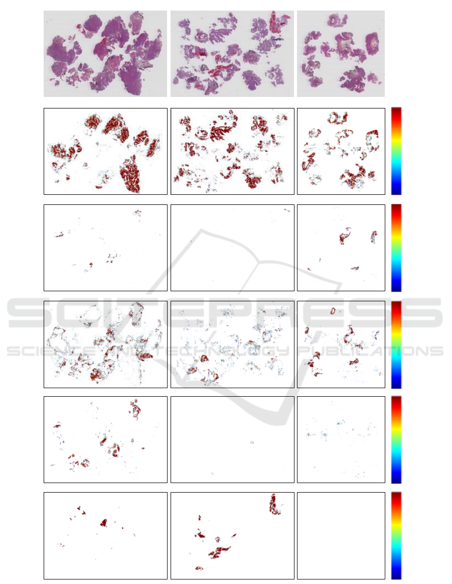
Original image

Stroma

Urothelium

Damaged

Blood

Muscle

0.8

1.0

0.9

0.8

1.0

0.9

0.8

1.0

0.9

0.8

1.0

0.9

0.8

1.0

0.9

Figure 3: The original WSI together with the corresponding heat maps. The scale in the rightmost column shows the con-

ﬁdence level given by the model. The background heat maps are performing very good, but has been omitted from the heat

map visualisation since it is just removing the borders between background and tissue. The heat maps have been smoothed

with a Gaussian ﬁlter and thresholded to only contain predictions of 0.8 and higher.

ICPRAM 2019 - 8th International Conference on Pattern Recognition Applications and Methods

326

death for 20 age groups in 1990 and 2010: a system-

atic analysis for the Global Burden of Disease Study

2010. The Lancet, 380(9859):2095–2128.

Mangrud, O. (2014). Identiﬁcation of patients with high

and low risk of progresson of urothelial carcinoma of

the urinary bladder stage Ta and T1. PhD thesis, Ph.

D. dissertation, University of Bergen.

Martinez, K. and Cupitt, J. (2005). Vips-a highly tuned im-

age processing software architecture. In Image Pro-

cessing, 2005. ICIP 2005. IEEE International Confer-

ence on, volume 2, pages II–574. IEEE.

Pedregosa, F., Varoquaux, G., Gramfort, A., Michel, V.,

Thirion, B., Grisel, O., Blondel, M., Prettenhofer,

P., Weiss, R., Dubourg, V., et al. (2011). Scikit-

learn: Machine learning in python. Journal of ma-

chine learning research, 12(Oct):2825–2830.

Sulimowicz, L. and Ahmad, I. (2017). “rapid” regions-

of-interest detection in big histopathological images.

In Multimedia and Expo (ICME), 2017 IEEE Interna-

tional Conference on, pages 595–600. IEEE.

Wang, D., Khosla, A., Gargeya, R., Irshad, H., and Beck,

A. H. (2016). Deep learning for identifying metastatic

breast cancer. arXiv preprint arXiv:1606.05718.

Yao, J., Boben, M., Fidler, S., and Urtasun, R. (2015).

Real-time coarse-to-ﬁne topologically preserving seg-

mentation. In Proceedings of the IEEE Conference

on Computer Vision and Pattern Recognition, pages

2947–2955.

Multiclass Tissue Classiﬁcation of Whole-Slide Histological Images using Convolutional Neural Networks

327