Assessing Sequential Monoscopic Images for Height Estimation of

Fixed-Wing Drones

Nicklas Haagh Christensen, Frederik Falk, Oliver Gyldenberg Hjermitslev and Rikke Gade

Aalborg University, Denmark

Keywords:

UAV, Drone, Free Height Estimation, Stereo Equation, Computer Vision, Feature Detection.

Abstract:

We design a feature-based model to estimate and predict the free height of a ﬁxed-wing drone ﬂying at altitudes

up to 100 meters above terrain using the stereo vision principles and a one-dimensional Kalman ﬁlter. We

design this using a single RGB camera to assess the viability of sequential images for height estimation, and

to assess which issues and pitfalls are likely to affect such a system. This model is tested on both simulation

data ﬂying above ﬂat and varying terrain, as well as data from a real test ﬂight. Simulation RMSE ranges from

10.7% to 21.0% of maximum ﬂying height. Real estimates vary signiﬁcantly more, resulting in an RMSE

of 27.55% of median ﬂying height of one test ﬂight. Best MAE was roughly 17%, indicating the error to

expect from the system. We conclude that feature-based detection appears to be too heavily inﬂuenced by

noise introduced by the drone and other uncontrollable parameters to be used in reliable height estimation.

1 INTRODUCTION

Measuring the altitude of a ﬁxed-wing drone can be

achieved in different manners. An often used appro-

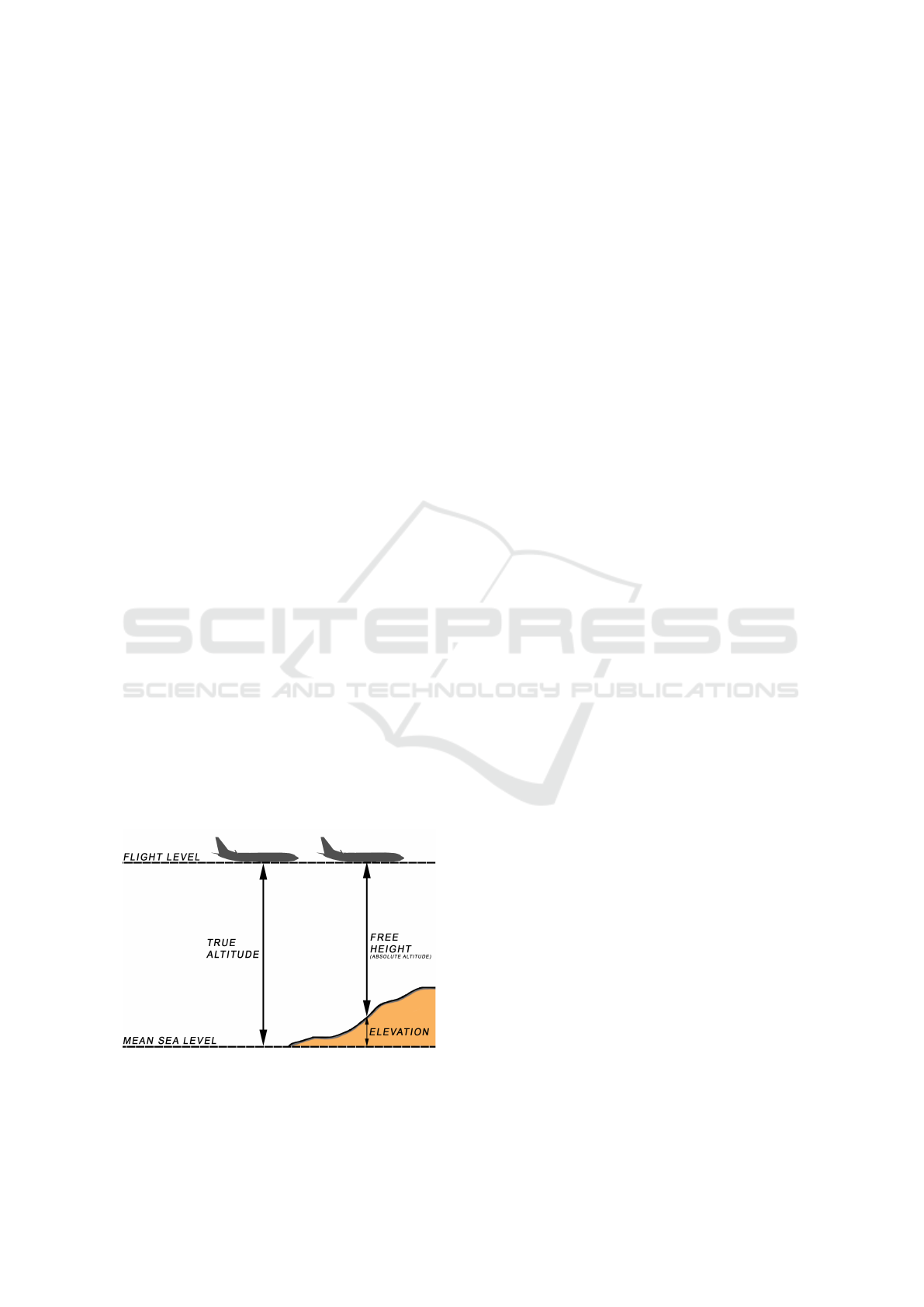
ach is by using a barometer or GPS altimeter. Free

height, or absolute altitude, is the measure of distance

from the drone to the terrain below. An illustration

can be seen in Figure 1. Most drones do not account

for obstacles or increasing/decreasing terrain as their

altitude is often measured relative to the drone’s take-

off point. Therefore, there is a need to estimate the

free height of drones, independent of their take-off

point, using other methods.

Figure 1: Figure illustrating the free height of a drone.

Other free height measurements exists, such as

ultra-sonic distance measurement or laser range ﬁn-

ders, but these are not sufﬁcient methods when ﬂying

at higher altitudes (> 100m) and would add additio-

nal weight to the drone as well as increasing energy

consumption as they are active sensors. As modern

drones are getting smaller and lighter, attaching addi-

tional sensors would decrease their efﬁciency. Since

many drones are already equipped with an RGB ca-

mera, a vision based solution is investigated to reduce

additional sensor weight. This is especially feasible

when using ﬁxed-wing drones as they travel in a spe-

ciﬁc direction and at relatively constant speeds. Ca-

meras provide rich information while still being low

on weight and energy consumption. Implementing vi-

sion based free height estimation would allow drones

to operate safely in areas with poor GPS coverage and

become independent of variations in air pressure. Cal-

culating the distance to the terrain below the drone

would also prove beneﬁcial in terrain with varying

ground level, and provide information necessary for

safe piloting.

2 RELATED WORK

Creating these estimates requires different approaches

in different contexts. Convolutional neural networks

have been capable of estimating depth with reasona-

ble accuracy in experimental set-ups given image data

(Eigen, 2014). This method has also shown to be able

Christensen, N., Falk, F., Hjermitslev, O. and Gade, R.

Assessing Sequential Monoscopic Images for Height Estimation of Fixed-Wing Drones.

DOI: 10.5220/0007256107510759

In Proceedings of the 14th International Joint Conference on Computer Vision, Imaging and Computer Graphics Theory and Applications (VISIGRAPP 2019), pages 751-759

ISBN: 978-989-758-354-4

751

to create a height map of a given image with no prior

information (Zhou et al., 2017).

However, using a downwards facing camera on

a drone enables the advantage of stereo correspon-

dence between sequential images. Previous work

has successfully implemented photogrammetric ae-

rial depth triangulation to estimate elevation or heig-

hts using vision (Schenk, 1997), (Hadjutheodorou,

1963), (Matthies et al., 1989), (Choi and Lee, 2012).

Using the stereo principle on sequential images from

the drone seems feasible to calculate the distance to

the ground based on the motion of the drone, as has

previously been done on rotor-drones (Campos et al.,

2016). This paper explores the possibility of enabling

automatic free height estimation using optical ﬂow

and stereo vision principles and calculate a reliability

measure for the operator on the ground. Investigating

similar work where computer vision has been used

for obstacle avoidance or mapping, the most common

methods used are optical ﬂow or SLAM based appro-

aches (Lu et al., 2018). Feature-based methods have

rarely been used despite its potential low cost. One

example of feature-based previous work is the use of

SIFT to detect obstacles by tracking size expansion

ratios in sequential images (Al-Kaff et al., 2016).

We therefore propose to evaluate feature-based

height estimation using a single monoscopic RGB ca-

mera in order to assess potential shortcomings and

error sources of such a system. A feature-based sy-

stem would not be affected by changing illumination,

which is an unavoidable aspect in the outdoors con-

text, and is more robust in handling sudden changes in

speed or rotation. The system will be suited to drones

operating above 100 meters, and assuming a relatively

constant ﬂight level. To this end, the existing sensors

on the drone can be used to retrieve the missing va-

riables, available from the drone’s inertial measure-

ment unit (IMU) and GPS. Based on these ﬁndings,

an evaluation should suggest potential pitfalls for fu-

ture works, and assess the viability of estimating free

height of a drone using a single RGB camera.

3 METHODS

We explore the use of the stereo equation in combi-

nation with feature detection and matching to calcu-

late the height of the drone and the reliability thereof

using sequential images from a downwards facing ca-

mera mounted to the drone. This section provides an

overview of the applied feature tracking, height esti-

mation, and reliability measure methods. The evalua-

tion approach and test methodology is also described

to clarify aspects such as drone data retrieval and ot-

her issues encountered through the process.

3.1 Feature Detection and Tracking

The system requires a method to detect robust fe-

atures that can be matched between sequential fra-

mes. Oriented FAST and Rotated BRIEF (ORB), was

chosen based on the speed of computation and rela-

tive robustness. Even though other methods such as

Scale Invariant Feature Transform (SIFT) are scale

invariant, ORB outperforms them in execution time

and with comparable accuracy allowing for real-time

tracking (Rublee et al., 2011).

ORB is a feature detector made for real-time

computations and low-power devices. It builds on

the Features from Accelerated Segment Test (FAST)

keypoint detector and a variant of the Binary Ro-

bust Independent Elementary Features (BRIEF) des-

criptor. The FAST method performs well in high

speed corner detection, by considering a circle of a

set amount pixels around a corner candidate. If the

brightness of these pixels are darker or brighter than

the candidate with a given threshold it is considered

a corner (Rosten et al., 2010). The BRIEF procedure

allows a shortcut in ﬁnding the binary strings without

having to ﬁnd the descriptors. It takes a smoothened

part of an image and ﬁnds a chosen amount of loca-

tion pairs. A pixel intensity comparison are done to

these pairs.

ORB employs a Harris corner ﬁlter to discard ed-

ges. FAST keypoints are computed with an orienta-

tion component, while BRIEF descriptors are consi-

dered rotation-invariant using steering according to

the orientation of the keypoints. According to the

authors, ORB performs as good as SIFT and better

than SURF on their evaluation data while being up

to factor-2 faster. Furthermore, ORB is derived with

the purpose of running in real-time or for low-power

systems. However, an issue with ORB, compared to

other feature detectors, is that it is not scale invari-

ant. As the drone used in this test is ﬂying at relati-

vely constant altitude between two frames, we assume

only little accuracy is missed from this. For applica-

tions where scale invariance is a necessity, computa-

tionally heavier solutions might be needed, such as

SIFT or SURF. As this is intended as an on-line solu-

tion for constant ﬂight level, the system beneﬁts from

the drone’s constant altitude by using less computati-

onally heavy feature detection.

With these arguments we hypothesize that ORB

is sufﬁcient to detect and track features for reliable

disparity calculations for use in height estimation.

VISAPP 2019 - 14th International Conference on Computer Vision Theory and Applications

752

3.2 Height Estimation

The height is calculated by using a calculation from

stereo vision and treating sequential images as stereo

vision with large baselines. Assuming two images are

taken with two cameras (left and right) with two dif-

ferent viewing positions the depth to the object can

be calculated by using the disparity between the same

object in the frames, the focal length, and the coordi-

nates of the object. For the left camera this is calcula-

ted as:

= f

(1)

As for the right camera:

= f

X − b

= f

(2)

This assumes that the object has moved in the x-axis

by a baseline b. x

and x

deﬁnes the pixel coordinates

of the object, whereas X is the real life coordinate,

same as Y. These two equations can be merged into

one explaining the effect of stereo disparity:

d = x

− x

= f

− ( f

− f

)

d =

f b

(3)

This equation can be rearranged to deﬁne the

depth (height) in the image:

Z =

f b

(4)

Where Z is the depth, f is the focal length, b is

the baseline, and d is the disparity in the image. This

equation will be referred to as the Stereo Equation.

Figure 2 displays the height estimation based on

these hypothetical values and shows the effect of the

cell size in the camera. Decreasing the cell size in-

creases the accuracy of the estimated height shown by

the smaller gradient of the red curve. It is important to

note that the height estimations with small disparities

(<5) generate increased uncertainty. For instance a

one-pixel displacement given similar values as above

would estimate a height between 1.25km and 625m,

whereas the next one-pixel displacement is between

625m and 416m.

This means that increasing disparity reduces the

range of the upper and lower bounds, indicating an

increased accuracy as the range decreases with one-

third for a two pixel displacement, one-fourth for

three pixels etc.

In order to perform these calculations, it is neces-

sary to know the drone’s rotation and speed, or GPS

Figure 2: The estimated height plotted as a function of dis-

placement in pixels using the hypothetical values; 20mm

focal length and 100mm baseline. Although pixels are dis-

crete values, they have been plotted as continuous for rea-

dability.

coordinates, at the time the images are captured to re-

liably calculate the baseline between images. In this

test, GPS data is available as embedded metadata in

the video, along with a range of other information.

3.3 Measurement Filters

As noise in the measurements is a reality and in order

to provide reliable and valid results, smoothing is ne-

cessary. Three ﬁlters were considered for smoothing

the calculated height using prior heights; a weighted

average, variable weighted average dependent on the

absolute pitch of the drone, and a Kalman ﬁlter. All

three approaches were tested, and the Kalman ﬁlter

(27.6% RMSE) was deemed most suited for the si-

tuation compared to both weighted average approa-

ches. The weighted average ﬁlter was tested substan-

tially, ranging from 0.9 of the last estimate to 0.99,

resulting in a higher minimum error than the Kalman

ﬁlter (27.9% RMSE) at 0.923. The variable weigh-

ted average was modelled based on the regular weig-

hted average approach. It decreased the last estimate

weight linearly dependent on the absolute pitch of the

drone, which ranges from 0 deg to roughly 40deg,

meaning high pitch values allowed the model to adapt

quicker. This was not enough to improve on the Kal-

man ﬁlter, resulting in an RMSE of 39.0%.

The Kalman ﬁlter parameters were determined by

internal testing described in Section 3.5.2. The as-

sumption was that the measurement noise variance

(σ

) could be described using the stereo equation,

as single pixel deviations can be modelled using the

Equation 5.

f B

−

f B

D + 1

(5)

Assessing Sequential Monoscopic Images for Height Estimation of Fixed-Wing Drones

753

Error Range (m)

Disparity

(pixels)

Baseline (m)

Error: 1.9m

Disparity: 10p

Baseline: 17m

Error: 0.2m

Disparity: 10p

Baseline: 2m

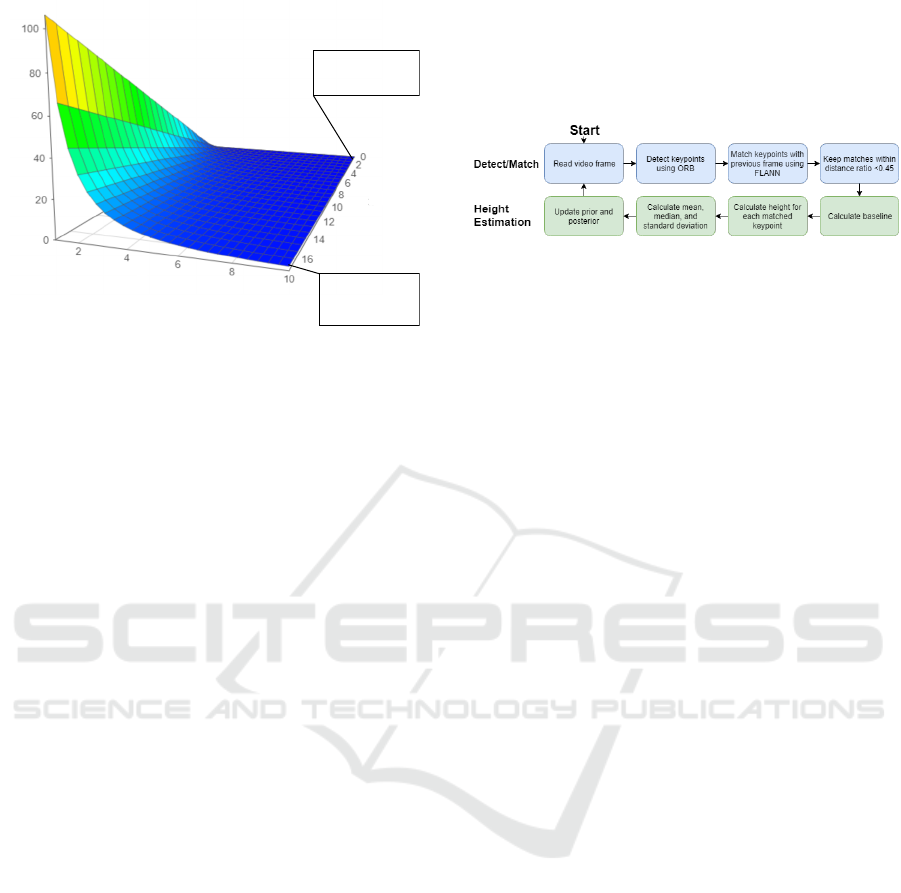
Figure 3: Relationship between disparity and baseline on

single pixel error.

This relationship is shown in Figure 3. The er-

ror decays exponentially with disparity and increases

linearly with baseline. Not only does this show that

the measurement error can be estimated relatively pre-

cisely, it also indicates that inﬁnitely decreasing the

baseline is a poor choice for optimizing the system,

since the disparity is dependent on the baseline but

with a much larger inﬂuence on measurement error.

This assumes that single pixel estimates are the

only measurement error we can reliably model. This

is true to the extent that more error sources are known,

but cannot be modelled for use in a Kalman ﬁlter. Ot-

her measurement errors include lens distortion, wind,

and GPS accuracy.

The model itself has a variety of errors inclu-

ding the pitch of the UAV, indifference to peripheral

keypoints, and importantly accuracy of keypoint mat-

ching. This error is denoted σ

for process noise vari-

ance. Some of these can be modelled mathematically,

for instance the relationship of the pitch and the dro-

nes altitude:

tan(θ)B (6)

Where the difference in altitude between frames

is dependent on the baseline of the drone and its pitch

θ. This, however, assumes that the drone has ﬂown

linearly between frames. Though this is not always

the case, it is relevant to understand why pitch has an

effect on the result.

Keypoint detection and matching will always be

an issue in such a naive model, since very close

keypoints result in a low disparity and a large estima-

ted height, however the error itself cannot be model-

led further than experimenting. As equally large ne-

gative and positive variance do not yield equally large

errors, the error cannot even be considered normally

distributed even if it could be predicted.

3.4 Algorithm

The algorithm was programmed in Python 3.6 and

follows the structure seen in Figure 4.

Figure 4: An overview of the program used to estimate the

free height of the drone.

It starts by detecting features in a frame using

ORB and then matches it with features from the previ-

ous valid frame using FLANN. This validity is deter-

mined as the video frame closest in recording time to

the last data-frame. The match must fulﬁll a distance

ratio lower than 0.45 before it is considered accep-

table. This is to ﬁlter out bad matches as shown in

Lowe’s paper on Scale-Invariant Feature Transforms

(Lowe, 2004). Furthermore, matches with keypoints

further than 50 pixels apart (on the ﬁxed axis, in our

case the x-axis) were discarded based on an internal

test comparing accuracy between 25, 50, 75, and 100

pixels.

The baseline is then calculated to be used in the

stereo equation and the height for each valid match is

calculated. The mean height for all matches is then

the estimated height for the current frame.

To avoid errors, some criteria have to be fulﬁlled

before the heights are used in the algorithm. If the

distance travelled is too small to be the result of ﬂight

or the frame-to-frame roll of the drone is too large,

the frame is discarded. This also applies if there are

fewer than ﬁve matches.

3.5 Experiments

This section describes the methods used to evaluate

the concept of using feature based computer vision

to calculate the height of the drone with a downward

facing camera. The outline of the evaluation is:

• Simulation above various terrain

• Error Variance Approximation

• Experiment with data from real drone

3.5.1 Simulation

A simulation of a drone ﬂying above virtual terrain

was created to test the concept of using feature ba-

sed stereo calculations with sequential images. This

VISAPP 2019 - 14th International Conference on Computer Vision Theory and Applications

754

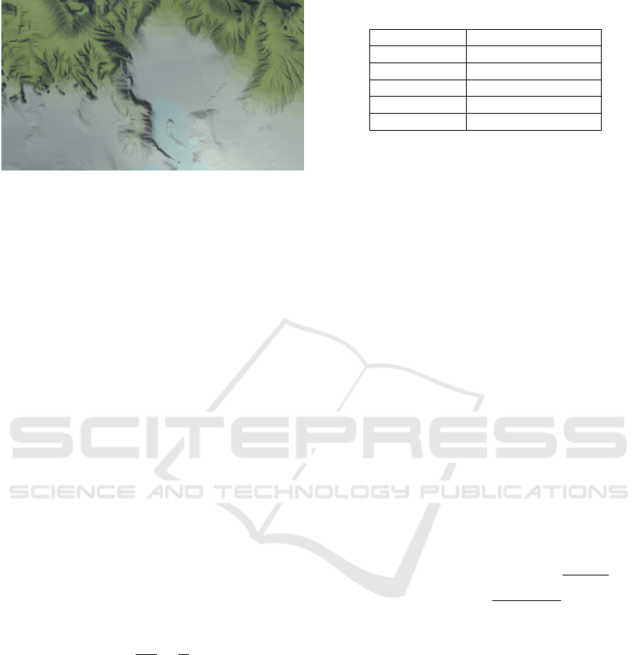
Figure 5: A frame from the simulation with 10 meter ground

truth.

approach has the advantages of controlling all the va-

riables and testing the system in near-ideal conditi-

ons without additional measurement and model er-

ror sources mentioned in Section 3.3. The simulation

data was created and recorded in Unity3D.

In total, 10 simulations were performed. Each tes-

ted optimal parameters for both σ

and σ

, and cal-

culated the best RMSE to compare with the test with

real data.

An image of one of the frames captured for the

simulation is seen in Figure 5. Multiple simulations of

different ground truths (i.e. the actual free height) are

needed to assess the viability of the system at different

heights.

3.5.2 Kalman Filter Parameter Estimation

All parameters described in 3.3 that could be reaso-

nable modelled were tested, as were combinations of

these. Additional constants and scalars were tested as

well, and results were observed for relations to pitch,

current height, baseline, etc. Finally, tests were made

solely with constant σ

and σ

Tests were performed using two loops, brutefor-

cing the best combination of the two variables. Both

variables were 0-centered and increased in small in-

crements ranging from

1000

Results were inspected to ensure the algorithm did

not ”cheat” in order to level at best results, but reaso-

nably followed the data provided.

3.5.3 Drone Experiment

Sky-Watch is a company that specializes in drones for

mapping of terrain and survey missions. They provi-

ded footage from their ﬁxed-wing drone for evalua-

tion purposes. These drones ﬂy in the range of 100m

to 1 km. There was approximately 30 minutes of

video including pre-ﬂight preparations, take-off, in-

ﬂight, landing, and drone retrieval. The footage con-

tained two separate ﬂights and was obtained using a

Table 1: Speciﬁcations of the camera used to record the

evaluation footage.

Model CM8359-B500SA-E

Sensor Size 3.6736 × 2.7384mm

Focal Length 2.759mm

Framerate 30 f ps

Data-rate ∼ 4/s

Resolution 1280 × 720

retired drone with an older camera. The speciﬁcations

of the camera can be seen in Table 1.

The footage was embedded with KLV metadata

which was extracted using FFmpeg. The parser was

written in Python. The resulting comma-separated va-

lues (CSV) ﬁle contained all relevant data for the test,

including the rotation of the drone, GPS-coordinates,

time stamp, heading, altitude, and azimuth. However,

the data rate was unstable, ranging from 2/s to 13/s.

An overview of the program used to estimate the

height is seen in Figure 4. Only the GPS-coordinates

and the rotation were used by the program, and the

relative altitude was used for ground truth. The ba-

seline was calculated by converting GPS coordinates

to longitude and latitude and calculating the euclidean

distance between.

The distance in latitude is in Equation 7, where

one degree latitude is 111.32 km.

lat =| lat

− lat

| ×111320000 (7)

With the difference in latitude, the total distance

travelled is calculated by ﬁnding the difference in lon-

gitude (Equation 8) and then use Pythagoras theorem

(Equation 9), assuming a straight line:

long =| long

− long

| ×40075km ×

cos(lat)

360

(8)

baseline =

lat

+ long

(9)

With the baseline calculated, each match’s asso-

ciated height is calculated using the stereo equation.

The resulting estimated height was compared to the

ground truth from the drone’s sensor. As the drone is

ﬂying above ﬂat terrain, this is deemed acceptable as

ground truth. The RMSE was calculated to compare

its reliability. Additionally, error rates such as mean

error (ME) and mean absolute error (MAE) was inves-

tigated to determine the accuracy users can expect.

Assessing Sequential Monoscopic Images for Height Estimation of Fixed-Wing Drones

755

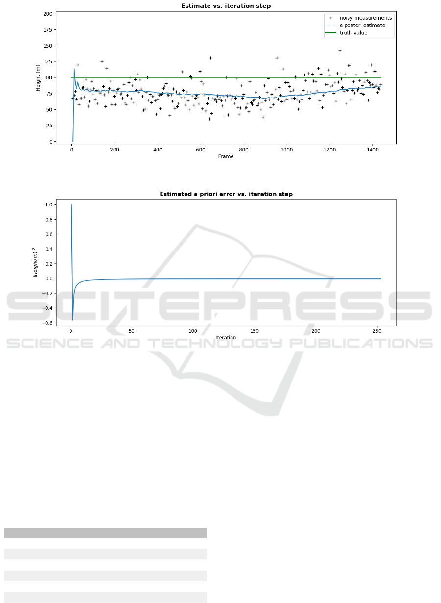
Figure 6: The estimated simulated heights at a constant 100m free height before and after ﬁltering.

Figure 7: A priori error before updating the measurements at 100m.

4 RESULTS

4.1 Simulation with a Flat Terrain

The ﬂat terrain tests consisted of 7 out of 10 total

simulation tests performed at heights of 10m, 20m,

30m, 40m, 50m, 75m, and 100m. An example simula-

tion is shown in Figures 6 and 7.

Table 2: Table describing the simulation RMSE, process

and measurement error, and the RMSE as a percentage of

ground truth.

Height RMSE % of truth σ

10m 1.78m 17.8 0.0036 1.0

20m 3.87m 19.4 0.0081 4.0

30m 3.64m 12.1 3.6 × 10

−5

0.25

40m 4.41m 11.0 0.0001 0.36

50m 5.35m 10.7 0.0001 0.25

75m 13.23m 17.6 0.0001 0.36

100m 21.02m 21.0 0.0002 0.36

Table 2 shows the estimated best error variances

and calculated best RMSE for each height.

The results indicate that there is no relationship

between height or baseline in the measurement or pro-

cess error variance. Instead, assuming constant error

variances produced the best results overall. This way,

RMSE seems to increase from roughly 10% to 20%

of free height at 100 meters.

4.2 Simulation with Varying Terrain

The varying terrain were tested at 3 maximum free

heights, 50m, 75m, and 100m. An example simulation

is shown in Figures 8 and 9.

All results are shown in Table 3. As with the

constant ﬂying height, there appears to be no obvious

correlation between either of the variables, but the

RMSE drops signiﬁcantly with the varying height.

This seems to be caused by the dips in free height,

VISAPP 2019 - 14th International Conference on Computer Vision Theory and Applications

756

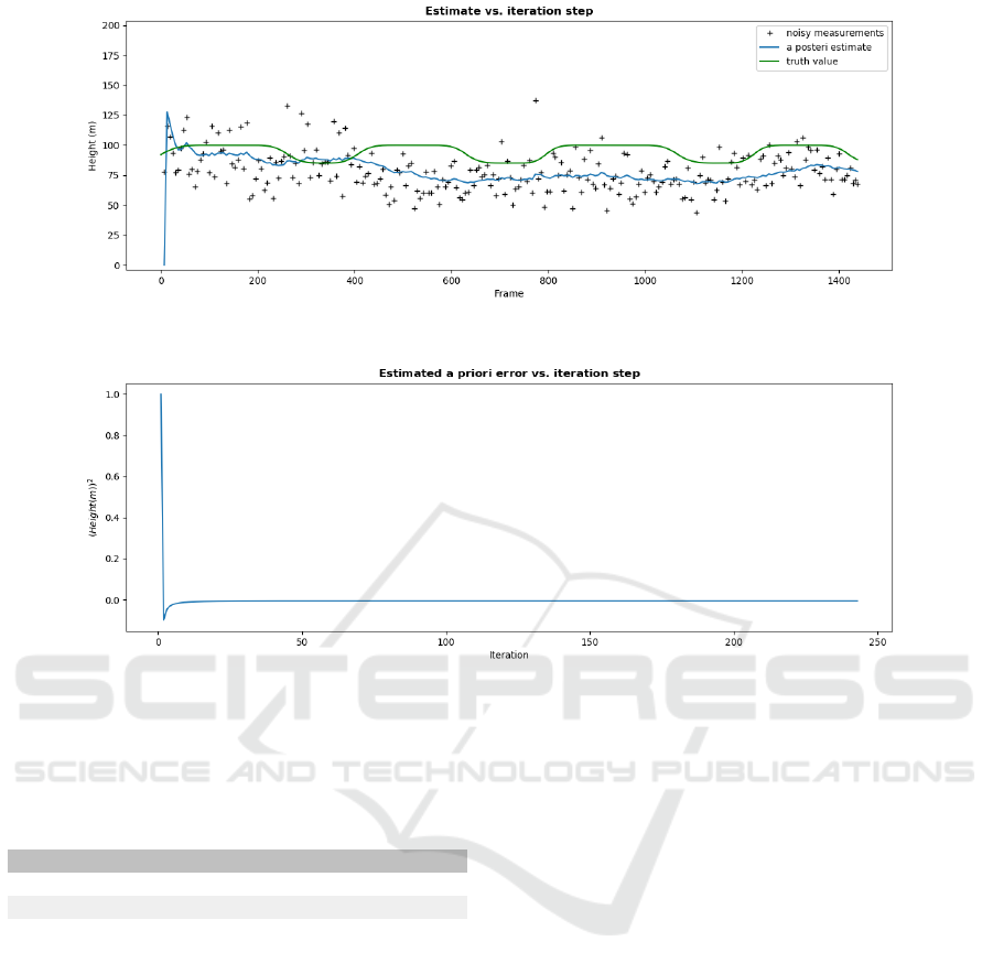
Figure 8: The estimated heights at a varying 100m free height before and after ﬁltering.

Figure 9: A priori error before updating the measurements at 100m varying heights.

since the model appears to underestimate the

height in both tests.

Table 3: Table showing the results for the simulations with

varying terrain.

Height RMSE (m) % of truth σ

50m 8.96 17.9 0.0076 25

75m 8.30 11.0 0.0035 1.69

100m 11.65 11.6 3.6 ∗ 10

−5

0.09

As mentioned previously, the estimates not increa-

sing signiﬁcantly at intervals of maximum free height

is likely due to the algorithm accepting peripheral

keypoints equally with centered ones.

4.3 Testing on Drone Data

When testing the algorithm on data from the real

drone ﬂying above a ﬂat terrain, the results become

noisier. This can be seen in Figure 10.

As seen in the Figure, the estimate follows the

ground truth to a certain degree, however is heavily

inﬂuenced by noise. This estimate results in a total

RMSE value of 27.1, a MAE of 17, and a ME of -

3. Some of this error can be attributed to the fact

that a delay in calculated height will always be pre-

sent when using ﬁltering methods such as Kalman.

Taking the mean of all standard deviations across all

included frames results in 58.6 meters which indicate

a lot of noise on the measurements. The negative ME

is in line with previous observations that the model

underestimates the actual height of the drone.

All previously mentioned factors such as pitch,

current height, and baseline, were tested as proba-

ble error variance sources, however none improved

on constant σ

and σ

. This is in line with simula-

tion tests, as well as the previous variable weighted

average test. Results of these one-dimensional noise

covariances are seen in Equation 10.

= 0.000441, σ

= 0.9604 (10)

Looking at Figure 11 reveals that some of the er-

ror might come from inaccurate GPS coordinates or

miscalculated distance. With a top speed of 60 km

per hour, and a datarate of 4 datasets per second the

drone should not be able to gain distances between

frames larger than 4.15 meters.

Assessing Sequential Monoscopic Images for Height Estimation of Fixed-Wing Drones

757

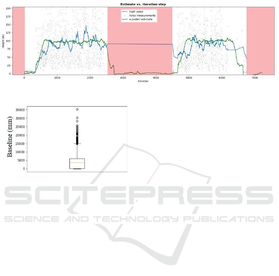
Figure 10: Ground truth, raw measurements and ﬁltered results. Red areas represents data not included in the calculations as

the drone is not ﬂying or no data was recorded.

Figure 11: Boxplot showing the calculated baselines for the

drone.

5 DISCUSSION AND

CONCLUSION

Comparing to simulations, data from a real drone is

much more inﬂuenced by noise and as such, measu-

ring height with a single camera does not translate

well from simulation to reality. Comparing to rela-

ted work, Campos et. al achieved MAE around 17%

(Campos et al., 2016). This is in line with our MAE

results using a relatively similar setup, however free

from abrupt stopping and starting, indicating a simi-

lar error range for current vision based free height es-

timators.

A lot of the error can be attributed to inaccurate

data such as using GPS coordinates for baselines and

roll and pitch of the drone. Another crucial part of this

approach is accurate disparity calculations, which is

affected by the chosen feature detector, camera qua-

lity, and terrain texture. In this example, ORB was

chosen for its effectiveness in real-time despite it not

being scale invariant. A scale-invariant feature detec-

tor might improve the results, but a method to run it

in real-time will be required.

Currently, systems such as these that rely on sin-

gle monoscopic cameras seem unfeasible to accura-

tely estimate a drone’s free height at any distance. The

main issue appears to be noisy data, for example poor

matches between the relatively simple ORB features,

discrepancies in data rate, and image quality (both re-

solution, color depth, and shaking). Some of these

can be solved by improving certain aspects of the har-

dware or algorithm, but camera shake and computati-

onal efﬁciency remain major obstacles for sequential

monoscopic real-time free height estimation.

This paper has explored some of the error sources

relating to feature-based height estimation using a sin-

gle camera and this approach does not appear feasible

for precise estimates with the current setup due to the

many error sources associated with a camera moun-

ted to a ﬁxed wing drone. However, it does show the

beginning of a trend for vision based free height es-

timation as an alternative to barometers or GPS, and

provides some indication for what future works could

improve upon.

ACKNOWLEDGEMENTS

We would like to thank Sky-Watch for their partici-

pation in the project and for providing footage for the

evaluation of our system, as well as Rikke Gade for

all her help with the project.

REFERENCES

Al-Kaff, A., Qinggang Meng, Martin, D., de la Escalera,

A., and Armingol, J. M. (2016). Monocular vision-

based obstacle detection/avoidance for unmanned ae-

rial vehicles. pages 92–97. IEEE.

Campos, I., Nascimento, E., Freitas, G., and Chaimowicz,

L. (2016). A Height Estimation Approach for Terrain

Following Flights from Monocular Vision. Sensors,

16(12):2071.

Choi, K. and Lee, I. (2012). A Sequential Aerial Tri-

angulation Algorithm for Real-time Georeferencing

VISAPP 2019 - 14th International Conference on Computer Vision Theory and Applications

758

of Image Sequences Acquired by an Airborne Multi-

Sensor System. Remote Sensing, 5(12):57–82.

Eigen, D. (2014). Depth map prediction from a single image

using a multi-scale deep network. Advances in neural

information processing systems, pages 2366–2374.

Hadjutheodorou, C. (1963). Elevations from Parallax Me-

asurements. Photogrammetric Engineering, 29:840–

849.

Lowe, D. G. (2004). Distinctive Image Features from Scale-

Invariant Keypoints. International Journal of Compu-

ter Vision, 60(2):91–110.

Lu, Y., Xue, Z., Xia, G.-S., and Zhang, L. (2018). A survey

on vision-based UAV navigation. Geo-spatial Infor-

mation Science, 21(1):21–32.

Matthies, L., Kanade, T., and Szeliski, R. (1989). Kal-

man ﬁlter-based algorithms for estimating depth from

image sequences. International Journal of Computer

Vision, 3(3):209–238.

Rosten, E., Porter, R., and Drummond, T. (2010). Faster

and Better: A Machine Learning Approach to Corner

Detection. IEEE Transactions on Pattern Analysis and

Machine Intelligence, 32(1):105–119.

Rublee, E., Rabaud, V., Konolige, K., and Bradski, G.

(2011). ORB: An efﬁcient alternative to SIFT or

SURF. pages 2564–2571. IEEE.

Schenk, T. (1997). Towards automatic aerial triangulation.

ISPRS Journal of Photogrammetry and Remote Sen-

sing, 52(3):110–121.

Zhou, X., Zhong, G., Qi, L., Dong, J., Pham, T. D., and

Mao, J. (2017). Surface height map estimation from

a single image using convolutional neural networks.

page 1022524.

Assessing Sequential Monoscopic Images for Height Estimation of Fixed-Wing Drones

759