RF Pulses Modelization for EMG Signal Denoising in fRMI Environment

Soﬁa Ben Jebara

Carthage University, Ecole Sup

erieure des Communications de Tunis,

COSIM Laboratory,

Route de Raoued 3.5 Km, Cit

e El Ghazala, Ariana, 2088, Tunisia

Keywords:

EMG Signal, fRMI, RF Pulses, HNM Model, Noise Reduction.

Abstract:

This paper deals with noise contaminating EMG signal acquired in fRMI environment. The RF pulses are

particularly addressed. Their characterization in the frequency domain allows their presentation as discrete

pulses repeated at frequencies multiple of RF pulses repetition. The Harmonic plus Noise Model (HNM) is

then used to model these pulses in the time-domain. The parameters of the model are extracted, frame by

frame, according to the principle of short time analysis. The model is validated according to two criteria: the

Segmental Signal to Noise Ratio (SSNR) and its Normalized Standard Deviation (NSD

SSNR

). Once modeled,

the estimated noise is subtracted from noisy observation of EMG signal, leading to an enhanced version.

Simulation results are given, validating the approach. In absence of ground truth, realistic situations are

simulated in order to calculate quantitative criteria. Furthermore, qualitative appreciation is given thanks to

muscular contractions proﬁles. Finally, the results are compared to those obtained with spectral subtraction

and comb ﬁltering.

1 INTRODUCTION

The acquisition of EMG signals simultaneously

with brain images in functional Magnetic Resonance

Imaging (fRMI) environment offers an added value

compared to acquisition of EMG signal outside the

scanner. In fact, the combination of the two modali-

ties allows to explore the dynamics of neural activity

and to link it to muscle response to the brain com-

mand. However, these advantages come with draw-

backs like artifacts: EMG data collected during fRMI

experiments are contaminated by artifacts due to tech-

nical and physiological origins. The cross talk (elec-

trodes over an adjacent muscle pick-up a signal via

skin conduction) is one common physiological arte-

fact, the EMG signal acquisition system (driver am-

pliﬁer, electrodes, cable movement,...) is one source

of technical artifact. In fRMI environment, the EMG

signal is affected by a supplementary noise which has

a very high level. It has two main origins: the very

high static magnetic ﬁeld (of the order of Tesla, which

corresponds to thousands of times the earth’s mag-

netic ﬁeld) and the ordered combination of RF and

gradient pulses designed to acquire the data to form

the image. The radio frequency pulses are emitted to

excite hydrogen nuclei for images generating while

magnetic ﬁeld gradients are introduced for spatial en-

coding of the image (see for example (Hornak, 2006)

for more details).

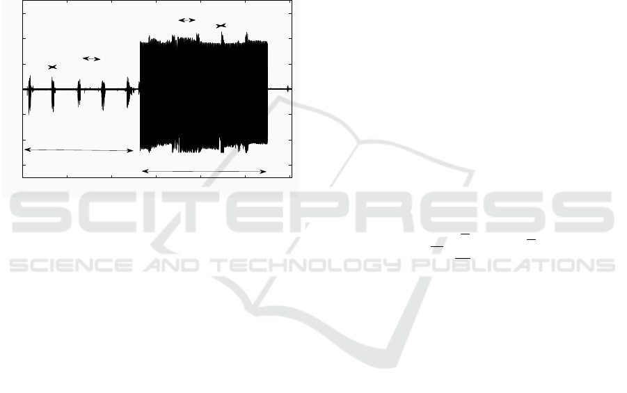
Fig. 1 shows an example of EMG data acquired in

normal conditions (outside the scanner) and in fRMI

environment (inside the scanner). Segment ’Noise

out’ (resp. ’Noise in”) corresponds to physiological

and technical noises (resp. physiological, technical

and speciﬁc fRMI noises) since there is no muscle ac-

tivity and the acquisition is carried outside (resp. in-

side) the scanner. Segment ’EMG out’ (resp. ’EMG

in’) corresponds to effective EMG signal during mus-

cle activity outside (resp. inside) the scanner. One can

notice the high level of noise due to radio-frequency

and gradient pulses. This noise completely buries the

EMG signal.

This paper aims at modelizing the RF pulses in

order to denoise EMG signals acquired in fRMI envi-

ronment. At the best of our knowledge, the mathemat-

ical modelization of fRMI noise did not attract the at-

tention of researchers, even though it is well analyzed

from a physical point of view and its origin and fre-

quency properties are well mastered (see for example

(Hoffmann et al., 2000)(Ganesh et al., 2007)(El Tatar,

2013)(Dougherty, 2010)(Garreffa et al., 2003)). In

this paper, we propose to develop an analytical model

of the RF pulses from observations when no prior in-

formation about RF pulses is available. The model

Ben Jebara, S.

RF Pulses Modelization for EMG Signal Denoising in fRMI Environment.

DOI: 10.5220/0007256401090115

In Proceedings of the 12th International Joint Conference on Biomedical Engineering Systems and Technologies (BIOSTEC 2019), pages 109-115

ISBN: 978-989-758-353-7

109

takes its origin from spectral characterization of noise

and leads to an Harmonic plus Noise Model (HNM).

This model will be exploited to denoise EMG signal

acquired in RMI environment.

The paper is organized as follows. Section 2 de-

scribes the RF noise in temporal and frequency do-

mains. Section 3 is devoted to HNM model expla-

nation and the algorithm to calculate its parameters.

Section 4 takes advantage of the model to reduce

noise from the EMG signal. Section 5 compares the

performances of proposed HNM model to Comb ﬁl-

tering and Spectral Subtraction technique. Finally,

conclusions are drawn.

700 800 900 1000 1100 1200

Time (s)

-6

-4

-2

EMG

Inside the scanner

Outside the scanner

Noise in

Noise out

EMG out

EMG in

Figure 1: Temporal evolution of EMG signal before and

during image acquisition in fRMI tunel.

2 RF NOISE PROPERTIES

2.1 Data Acquisition

Participants were lying in the fRMI scanner with fore-

arm connected to bipolar electrodes (ADD208, 8-mm

recording diameter, System Inc., Santa Barbara, CA).

Surface EMG signals were recorded during a hand-

grip exercice from the Flexor Digitorum Superﬁcialis

(FDS) muscle. Simultaneously, neuro-imaging data

were acquired with an MRI system. The RF pulses

and the gradient ﬁelds are applied repetitively to ac-

quire image slices of the brain. One loop, for com-

plete brain volume scan, occurs during a time interval

called repetition time (denoted T

). One loop allows

to generate a sequence of images (slices). Each image

is obtained during one RF stimulation period. The du-

ration between two RF pulses T

is equal to the repeti-

tion time T

over the number of slices N: T

= T

/N.

2.2 RF Pulses Properties

To study the inﬂuence of the noise generated by RF

pulses in the EMG signal, let’s consider some exam-

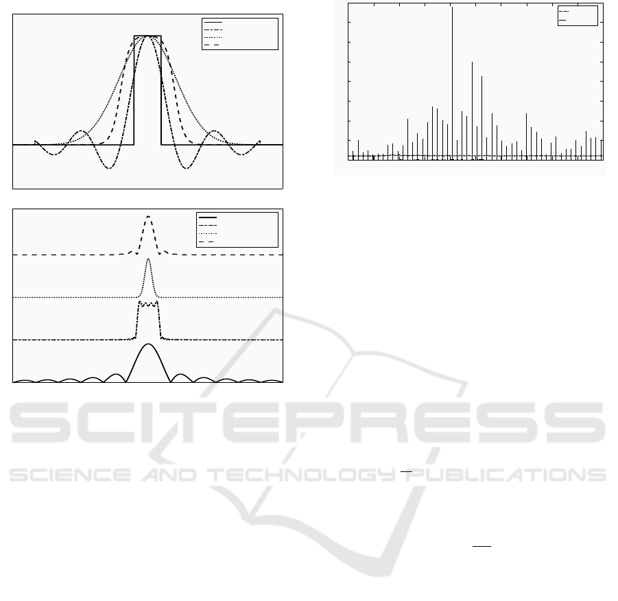
ples of RF pulses commonly used in practice. Fig. 2

gives time-continous temporal evolution (a) and spec-

trums (b) of some common RF pulses, namely rect-

angle, windowed sinus cardinal, Gaussian and Fermi

(Bernstein et al., 2004). Note that only the active part

(non null part) is drawn and ﬁgures axis are not given

in order to focus only on the shape. All the pulses are

time-limited. In the frequency domain, the Gaussian,

the windowed sinus cardinal and Fermi pulses are

characterized by band-limited spectrum while rectan-

gular pulse is characterized by an inﬁnite frequency

support.

The RF pulses are repeated periodically in order

to acquire the whole image slices of the brain. Let’s

denote x(t) the RF pulse. According to its periodicity

property, its Fourier transform is a sum of dirac pulses

equally spaced in the frequency axis at frequencies

multiple of f

X( f ) =

∑

k∈Z

δ( f − k f

), (1)

where X

is the k

Fourier transform coefﬁcient, cal-

culated during one period according to the following

formula:

−T

x(t)e

− j2π

dt. (2)

The RF analog signal is converted to a digital one.

When sampled and according to Shannon theorem, a

spectral overlap can appears due to the duplication of

the spectrum around the multiples of the sample fre-

quency:

Xs( f )

= f

∑

l∈Z

X( f − l f

) = f

∑

k∈Z

∑

l∈Z

δ( f − l f

− k f

(3)

With an appropriate choice of the parameters of

the RF pulse, their bandwidth can be adjusted so

that the duplication of spectrum around sampling fre-

quency multiples allows to reduce/avoid overlapping.

While windowed sinus cardinal, Gaussian and Fermi

RF pulses can lead to non-overlapping (thanks to their

band-limited spectrum), the rectangle pulse generates

overlapping (because of its inﬁnite frequency sup-

port). An alternative solution is to increase the sam-

pling frequency so that the overlap becomes less im-

portant (since the secondary lobes vanish when the

frequency increases). But increasing the sampling

frequency increases the number of samples acquired,

which is not necessarily interesting in term of data

amount.

BIOSIGNALS 2019 - 12th International Conference on Bio-inspired Systems and Signal Processing

110

(a)

Rectangle

Windowed Sinc

Gaussian

Fermi

(b)

Rectangle

Windowed Sinc

Gaussian

Fermi

Figure 2: Some common RF pulses. Spectrums are shifted

for better legibility.

2.3 RF Pulses Properties as Noise in

EMG

To deal with a concrete example, we consider the case

where the repetition time is equal to T

= 2215ms and

N = 43 images are acquired. The frequency of repeti-

tion of RF pulses is f

= 1/T

= 9.706 Hz. The signal

of interest is the EMG signal of FDS muscle. Its max-

imum frequency is 500 Hz so that it should be ideally

sampled at 1 kHz. The RF interference acquired as

noise in EMG is sampled at the same frequency.

Fig. 3 shows the spectrum of noise generated

during real acquisition in the RMI tunnel (according

to the protocol described in subsection 2.1). Note

that frequency bins due to RF noise exist along the

whole frequency axis at frequencies multiple of f

9.706Hz. Their amplitudes differ from one frequency

to another. This noise spectrum is compared to the

one of an EMG signal which looks like a white noise

with relatively very low level compared to that of RF

pulses. Hence, the challenging task is to estimate this

noise and to reduce it.

0 50 100 150 200 250 300 350 400 450 500

Frequency (Hz)

100

200

300

400

500

600

700

800

Spectrum

RF pulses

EMG

Figure 3: Spectrum of EMG signal and noise generated dur-

ing a real acquisition in the RMI tunnel.

3 RF PULSES MODELISATION

Eq. 3 describes digital RF pulses as a weighted sum of

frequency bins. Hence, in time-domain, we propose

to model the periodic RF pulses as a weighted sum of

sine waves:

˜x(m) =

K−1

∑

k=0

(m)sin(2πkν

m + φ

(m)), (4)

where ˜x(m) is the modeled sample at time index

m, K is the number of harmonics. For each harmonic

k, a

(m) and φ

(m) represent the time-varying ampli-

tude and phase respectively. ν

is the normalized fre-

quency ν

. The number of harmonics is equal

to the nearest integer of the signal maximal frequency

( f s/2) over the fundamental frequency f

K = b

f s

2 f

c. (5)

For our practical case, the EMG signal is sampled

at f

= 1 kHz and RF fundamental frequency is f

9.706, so the number of harmonics is K = 51.

3.1 Model Parameters Calculs

To estimate the parameters of the model, the follow-

ing methodology is adopted. It is inspired from pre-

vious works developed on speech processing (see for

example (Pantazis, 2010)).

• In the RMI tunnel, the RF pulses generator is

turned on. EMG signals acquisition are placed on

the considered muscle and the subject is asked to

not do any muscular activity. The EMG acquisi-

tion system is turned on so that the acquired signal

is the environmental noise. It is composed of tech-

nical and physiological artefacts, static magnetic

ﬁeld, RF pulses and gradient ﬁelds.

RF Pulses Modelization for EMG Signal Denoising in fRMI Environment

111

• Short-term analysis is done. The recorded signal

is decomposed into frames of length N and is win-

dowed using Hanning window for example. The

frame by frame analysis allows to assume that am-

plitudes and phases of the harmonics are constant

within a frame. The choice of the frame size will

be discussed later.

Let’s denote x

(u) the u

sample (u = 0,..N − 1)

belonging to the frame number l of the signal.

• The frequency f

of RF pulses could be known

from the RMI scanner datasheet. Otherwise, it can

be estimated using any precise method of period-

icity measure or by spectrum peak picking. The

estimated normalized frequency is denoted

• Each frame is converted to the analytic complex

signal using the Hilbert transform. It is denoted

(u).

• The estimation of the amplitudes a

k,l

and the

phases φ

k,l

of each harmonic k, for each frame

l is performed by minimizing the Least Squared

(LS) error between the Hilbert transformed signal

(u) and the Hilbert transformed modeled RF

noise

(u):

(u) = x

(u) −

(u)

= x

(u) −

K−1

∑

k=0

k,l

(

2πk

k,l

)

. (6)

where

k,l

and

k,l

are the parameters to be deter-

mined.

• Minimizing the Least Square error leads to the

following solution:

= (M

W M)

−1

W X

, (7)

where T is the transpose operator, X

(0),x

(1),...,x

(N − 1)]

is the vector of

Hilbert transformed samples, W is the analyzing

window vector of length N, M is a matrix of di-

mension N × K containing the exponential terms

M(l,k) = e

j2π

= [

0,l

1,l

,...,

K−1,l

]

is the

unknown vector of parameters.

One term

k,l

is written:

k,l

cos



k,l



− j

k,l

sin



k,l



. (8)

The ﬁnal solution is

k,l

extracted as the modulus

k,l

and

k,l

which is its phase.

• Once the parameters estimated, the RF pulse

frame is written:

(u) =

K−1

∑

k=0

k,l

cos



2πk

l +

k,l



. (9)

• The whole estimated signal

x(m) is estimated by

concatenating estimated frames.

0 500 1000 1500 2000 2500 3000 3500 4000

Frame duration (ms)

18.5

19.5

20.5

Normalized Standard Deviation

Segmental Signal to Noise Ratio (dB)

0.1

0.2

0.3

0.4

0.5

Segmental Signal to Noise Ratio

Normalized Standard Deviation

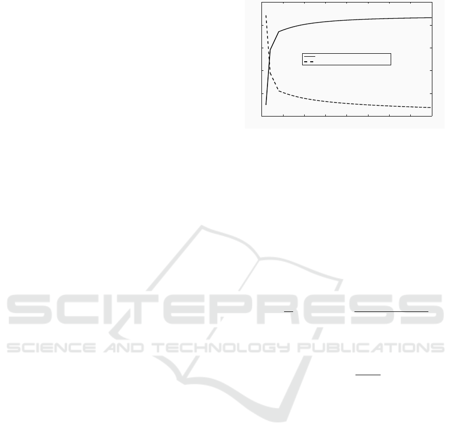
Figure 4: Segmental Signal to Noise Ratio and Normalized

Standard Deviation versus frame length.

3.2 Frame Size Choice

The choice of frame size is crucial to obtain good RF

pulse modelization. Two criteria are used to quantify

the performances: the Segmental Signal to Noise Ra-

tio (SSNR) which is the mean value of the SNR (in dB)

calculated for each frame and its Normalized Stan-

dard Deviation (NSD

SSNR

), useful to put into propor-

tion the SSNR deviation along frames compared to its

mean. The two criteria are deﬁned as follows:

SSNR =

∑

l=1

10log10







∑

u=1

(u)

∑

u=1

(u) −

(u)]







(10)

and

NSD

SSNR

, (11)

where σ

SSNR

(resp. m

SSNR

) is the SSNR standard

deviation (resp. mean) and M is the total number of

frames. Fig. 4 plots the evolution of both criteria for

different frame lengths. One can see that SSNR in-

creases and NSD

SSNR

decreases when frame length

increases. It means that better modelisation is ob-

tained for longer frames. However, the rate of im-

provement begins to stabilize around a frame size of

one second. This duration is considered adequate for

this study.

4 INTEREST IN EMG SIGNAL

DENOISING

4.1 The Idea

One RF pulse modelled, it is possible to reduce its ef-

fect on acquired EMG signal when RMI scanning is

BIOSIGNALS 2019 - 12th International Conference on Bio-inspired Systems and Signal Processing

112

turned on and when the subject is activating its mus-

cle and doing the requested muscular exercice. The

corrupted EMG signal y(m) can be presented as the

sum of the muscle signal emg(m), the RF signal x(m)

and any other additive noises n(m):

y(m) = emg(m) + x(m) + n(m). (12)

The enhanced emg signal should be simply obtained

by subtracting the modeled RF signal

s(m) from the

observation y(m):

emg(m) = y(m) −

x(m). (13)

Note that other additive noises are not yet consid-

ered during this step, because of their low level com-

pared to that of RF noise. Common technical artifacts

can be reduced, in a post processing stage, using other

approaches (see for example (Thakor and Zhu, 1991)

for reducing power line electrical noise, (Lu et al.,

2009) to suppress electrocardiogram (ECG) interfer-

ence, (De Luca et al., 2010) to remove noise associ-

ated to mechanical perturbations...).

4.2 Illustration

When acquired, the EMG signal is buried in noise and

there is no ground truth to quantitatively measure the

performance. The idea developed here is to compare

the signal with a reference which could be the sig-

nal acquired out of scanner. Hence, the same partici-

pant is asked to do the same handgrip exercice inside

and outside scanner according to the same experimen-

tal paradigm. In each case, he did 15 contractions of

duration 4.4 seconds approximatively, separated by a

rest time of 44 seconds.

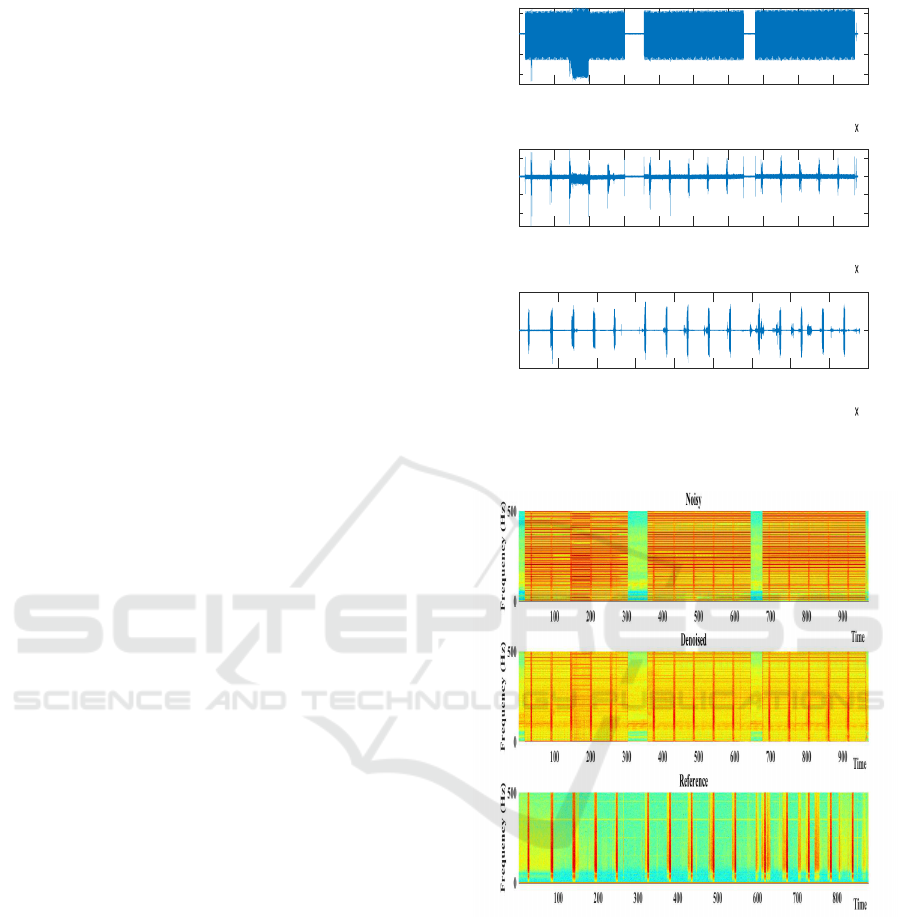
Fig. 5 (resp. Fig. 6) shows the temporal evolu-

tion (resp. spectrogram) of an EMG signal acquired

in the fRMI environment described previously, the

denoised one using the proposed approach and the

acquired EMG outside the scanner (called the refer-

ence). One can notice that EMG signal emerges from

noise despite the presence of small residual noise, and

the contractions have the same aspect as the ones of

the reference.

5 PERFORMANCES AND

COMPARISON

5.1 Overview on Comb Filtering and

Spectral Subtraction Methods

According to the state of art, few methods are devel-

oped to extract RF pulses from physiological signals

0 1 2 3 4 5 6 7 8 9 10

-4

-2

Noisy

0 1 2 3 4 5 6 7 8 9 10

-2

-1

HNM

0 1 2 3 4 5 6 7 8 9

Time (ms)

-1

Reference

Figure 5: Temporal evolution of noisy, denoised and refer-

ence EMG signals.

Figure 6: Spectrograms of noisy, denoised and reference

EMG signals.

acquired in RMI tunnel. The most common approach

is based on Comb ﬁltering (see for example (Ganesh

et al., 2007)). It operates in the temporal domain and

makes use of a digital ﬁlter which cancels frequency

components situated at frequencies multiple of funda-

mental frequency of RF pulses while keeping intact

the other frequencies.

Another approach is based on spectral subtraction

(see for example (Ben Jebara, 2014)). It operates

in the frequency domain to estimate the noise spec-

trum and to subtract it from noisy observation spec-

trum. The noise estimation is based on spectral min-

RF Pulses Modelization for EMG Signal Denoising in fRMI Environment

113

ima tracking in each frequency bin without any dis-

tinction between muscle activity and muscle rest. But

it looks for connected time-frequency regions of mus-

cle activity presence to estimate a bias compensation

factor. The proposed approach denoted HNM (Har-

monic plus Noise Model) is compared to spectral sub-

traction and Comb ﬁltering.

5.2 Comparison Criteria

To compare the methods, two criteria are used. The

ﬁrst one is quantitative and has the form of Mean Sig-

nal To Noise Ratio (MSNR) while the second one is

qualitative and uses the contraction proﬁle.

• The MSNR is calculated as a mean value of 285

SNR values obtained by studying FDS muscle

contractions made by 19 subjects, each repeating

the action 15 times. One SNR is calculated by tak-

ing data from a clean EMG signal acquired out-

side the tunnel. An additive real fRMI noise, ac-

quired in fRMI tunnel without exercing any con-

traction, was added by varying its level (artiﬁcial

attenuation and ampliﬁcation). Thus, it is possible

to calculate noisy MSNR (denoted MSNR

Noisy

)

and one MSNR at the output of the denoiser (de-

noted MSNR

Denoised

• The contraction proﬁle is a visual criteria used to

evaluate the quality of denoising. It is obtained

thanks to the Root Mean Square signal which is

a technique for rectifying the raw signal and con-

verting it to an amplitude envelope. It is deﬁned

as follows:

RMS(m) =

N/2−1

∑

n=−N/2

x(m + n)

, (14)

where x(n) is the m

sample of the signal on in-

terest and L is the length of the rectifying window.

It is chosen equal to L = 512 for a sampling fre-

quency of f

= 1kHz.

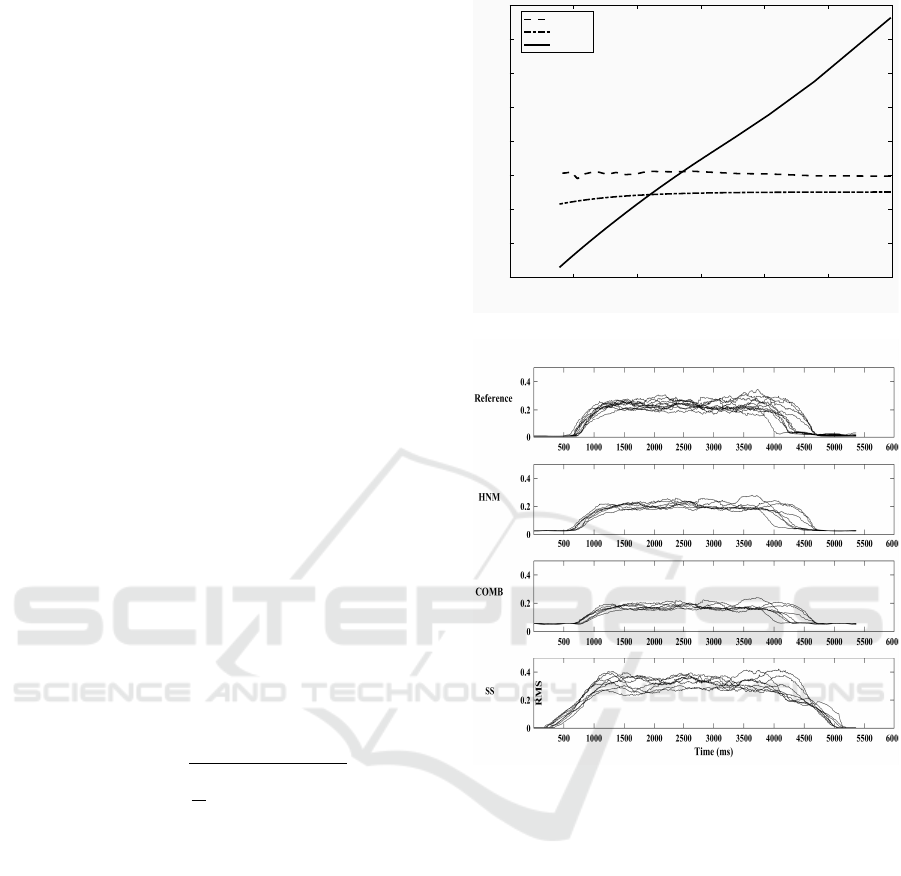
5.3 Results

Fig. 7 shows the evolution MSNR

Denoised

for different

values of MSNR

Noisy

ranging from -16 dB to 10 dB

dB. One can notice that, unlike HNM whose perfor-

mances vary according to the level of noise, Comb ﬁl-

tering and spectral subtraction lead to quasi-constant

values of MSNR

Denoised

, independently of the noise

level. Furthermore, Comb ﬁltering and spectral sub-

traction give better MSNR

Denoised

for high level of

noise (MSNR

Noisy

< -7 dB) while HNM performs for

greater values of MSNR

Noisy

-20 -15 -10 -5 0 5 10

MSNR

Noisy

-2

MSNR

Denoised

COMB

HNM

Figure 7: Evolution of MSNR

Denoised

versus MSNR

Noisy

Figure 8: Contractions proﬁle.

If we consider a real acquisition system: Biopac

MP150 system to digitize EMG data and General

Electric Medical System 3-Tesla whole-body MRI

system to generate RF pulses, a typical value of

MSNR

Noisy

is in the range [0 1] dB. In such case,

HNM should be used.

Fig. 8 draws the contraction proﬁles for the ref-

erence signal acquired outside the scanner and the

ones obtained after denoising. It is important to notice

that the contraction durations are not exactly the same

even though the volunteers were asked the follow the

same paradigm. The contraction durations are artiﬁ-

cially contracted/expanded in time so that comparison

is confortable. Fig. 8 shows that contractions proﬁles

are well restored. Their level is attenuated with comb

ﬁltering, their duration (at the beginning and at the

end) is extended with spectral subtraction. It seems

that HNM gives the best proﬁle.

BIOSIGNALS 2019 - 12th International Conference on Bio-inspired Systems and Signal Processing

114

6 CONCLUSION

In this paper, the problem of RF pulses noise contam-

inating the EMG signal acquired in fRMI scanner is

addressed. Thanks to its description in the frequency

domain and to its modelization using Harmonic plus

Noise model, it was possible to subtract it from EMG

signal, rmaking it exploitable for further analysis and

processing.

ACKNOWLEDGEMENTS

The authors are thankful to the team ’Biomechan-

ics, Imagery and Physiology Movement Analysis’ of

Movement and Sport Research Centre (CeRSM) at

Paris 10 University, for asking the resolve the problem

of EMG enhancement and providing the experimental

data.

REFERENCES

Ben Jebara, S. (2014). Electromyogram signal enhance-

ment in frmi noise using spectral subtraction. In

Proceedings of the 22nd European Signal Processing

Conference, pages 1980–1984.

Bernstein, M. A., King, K. F., and Zhou, X. J. (2004).

Handbook of MRI pulse sequences. Elsevier.

De Luca, C. J., Gilmore, L. D., Kuznetsov, M., and Roy,

S. H. (2010). Filtering the surface emg signal: Move-

ment artifact and baseline noise contamination. Jour-

nal of biomechanics, 43(8):1573–1579.

Dougherty, J. B. (2010). A novel and comprehensive artifact

reduction strategy for EMG collected during fMRI at

3 Tesla. PhD thesis, Drexel University.

El Tatar, A. (2013). Caract

erisation et mod

elisation

des potentiels induits par les commutations des

gradients de champ magn

etique sur les signaux

electrophysiologiques en IRM. PhD thesis, Universit

de Technologie de Compi

egne.

Ganesh, G., Franklin, D. W., Gassert, R., Imamizu, H., and

Kawato, M. (2007). Accurate real-time feedback of

surface emg during fmri. Journal of neurophysiology,

97(1):912–920.

Garreffa, G., Carnı, M., Gualniera, G., Ricci, G., Bozzao,

L., De Carli, D., Morasso, P., Pantano, P., Colonnese,

C., Roma, V., et al. (2003). Real-time mr artifacts ﬁl-

tering during continuous eeg/fmri acquisition. Mag-

netic resonance imaging, 21(10):1175–1189.

Hoffmann, A., J

ager, L., Werhahn, K., Jaschke, M.,

Noachtar, S., and Reiser, M. (2000). Electroen-

cephalography during functional echo-planar imag-

ing: detection of epileptic spikes using post-

processing methods. Magnetic Resonance in

Medicine: An Ofﬁcial Journal of the Interna-

tional Society for Magnetic Resonance in Medicine,

44(5):791–798.

Hornak, J. P. (2006). The basics of mri. http://www. cis. rit.

edu/htbooks/mri.

Lu, G., Brittain, J. S., Holland, P., Yianni, J., Green, A. L.,

Stein, J. F., and Wang, S. (2009). Removing ecg noise

from surface emg signals using adaptative ﬁltering.

Neuroscience letters, 462(1):14–19.

Pantazis, Y. (2010). Decomposition of AM-FM signals with

applications in speech processing. PhD thesis, Uni-

versity of Crete.

Thakor, N. V. and Zhu, Y.-S. (1991). Applications of adap-

tive ﬁltering to ecg analysis: noise cancellation and

arrhythmia detection. IEEE Transactions on biomedi-

cal engineering, 38(8):785–794.

RF Pulses Modelization for EMG Signal Denoising in fRMI Environment

115