Implementation of Trajectory Planning for Automated Driving Systems

using Constraint Logic Programming

Christian Wriedt

and Christoph Beierle

Audi Electronics Venture GmbH, Sachsstr. 20, 85080 Gaimersheim, Germany

Department of Computer Science, FernUniversit

at in Hagen, 58084 Hagen, Germany

Keywords:

Constraint Logic Programming, Trajectory Planning, Automated Driving Systems, ADAS, Autonomous

Driving, Explainable AI.

Abstract:

Automated driving systems are a maturing technology that is considered to have a signiﬁcant impact on

mobility. Trajectory Planning is a safety-critical task that plays an important role in automated driving

systems. In this paper, we present the implementation of a trajectory planning module called CLPTP

(CLPTRAJECTORYPLANNER) using constraint logic programming (CLP) and evaluate it in simulated traf-

ﬁc situations. CLP allows us to express the constraints of the problem of trajectory planning in a declarative

way. The approach makes the code less complex and more readable for domain experts compared to code

using an imperative programming language. Compared to approaches making use of neural networks to man-

age the complexity of the problem of trajectory planning, the results of CLPTP are more comprehensible and

easier to verify. Thus CLPTP can be seen as a step towards solving the problem of trajectory planning with

explainable artiﬁcial intelligence. An evaluation of the execution time performance of our implementation

shows that further research is needed to apply the approach in real world vehicles.

1 INTRODUCTION

In the past few decades, the level of automation in

road vehicles has been steadily increasing, result-

ing in a signiﬁcant decrease of trafﬁc accidents (ITF,

2017). Not only safety, but also accessibility, con-

venience and efﬁciency of automotive mobility are

expected to be enhanced by automated driving sys-

tems (Paden et al., 2016; Arbib and Seba, 2017).

Although many different automated driving sys-

tems are known to exist in research and development

projects, most of them share a similar functional ar-

chitecture in which the driving task is split in three

parts: Perception, decision and control, vehicle plat-

form manipulation (Behere and T

orngren, 2015). De-

cision and control is typically divided into three lev-

els: route planning, behavioural decision making and

trajectory planning (Paden et al., 2016).

It is the responsibility of the trajectory planning

level to ﬁnd a safe, comfortable and dynamically fea-

sible trajectory for the vehicle in its dynamic envi-

ronment. Due to space limitations, this paper focuses

on trajectory planning. Other related problems such

as object movement prediction or trajectory execution

are not discussed in this paper. The problem of trajec-

tory planning can be formulated as an optimization

problem with constraints imposed by trafﬁc rules, the

dynamic environment, vehicle dynamics etc. Many

algorithms have already been developed for solving

this problem. Some of them represent vehicle states

in the form of a graph and use search algorithms like

A* (Hart et al., 1968) for ﬁnding a minimum cost path

on the graph (Ziegler and Stiller, 2009; Gu and Dolan,

2012). Other solutions describe trajectories as poly-

nomials that are optimized under consideration of a

cost functional (Werling, 2011; McNaughton, 2011;

Kelly and Nagy, 2016; Rathgeber, 2016). Aside from

that, there are other implementations e.g. based on

neural networks and reinforcement learning (Dubey

et al., 2013; Zuo et al., 2014; Grigorescu et al., 2017).

Refer to (Paden et al., 2016) for a detailed presenta-

tion of the trajectory planning problem and an exten-

sive survey of motion planning techniques for self-

driving vehicles.

Translating the aforementioned constraints of the

problem of trajectory planning into software code can

be a challenging task when using imperative program-

ming languages because the speciﬁcation of the con-

straints are often present as declaratively written re-

quirements in natural language or in formal or semi-

Wriedt, C. and Beierle, C.

Implementation of Trajectory Planning for Automated Driving Systems using Constraint Logic Programming.

DOI: 10.5220/0007257904110418

In Proceedings of the 11th International Conference on Agents and Artiﬁcial Intelligence (ICAART 2019), pages 411-418

ISBN: 978-989-758-350-6

411

formal notations. Moreover, operational details in im-

perative code make it hard to read for domain experts

and more difﬁcult to verify, which is an important as-

pect for safety-critical software. Approaches using

neural networks overcome the challenging program-

ming task by learning desired planning behaviour

implicitly. However, verifying neural networks for

safety-critical systems, where international standards

such as ISO 26262 (ISO, 2011) must be applied, is

still an open problem (Grigorescu et al., 2017).

In this paper, we present the design and implemen-

tation of a trajectory planning module called CLPTP

(CLPTRAJECTORYPLANNER). CLPTP uses con-

straint logic programming (CLP), a programming

paradigm enhancing the declarative paradigm of logic

programming by mechanisms for specifying and solv-

ing constraints. By using this programming paradigm

with its high level of abstraction, program code is ex-

pected to be easier to understand and more concise

than its imperative counterpart. The planning results

are expected to be more comprehensible and easier

to verify than the output of a neural network, thus

supporting the trend for explainable artiﬁcial intelli-

gence (Biran and Cotton, 2017) with a different ap-

proach than e.g. (Bojarski et al., 2017).

Logic programming has already been used in (Pi-

aggio and Sgorbissa, 2000) for the symbolic compo-

nent of an autonomous robot navigator. CLP has been

successfully used to implement programs for solving

general planning and optimization problems (Lever

and Richards, 1994; Apt and Wallace, 2006). How-

ever, no attempt to apply CLP to the speciﬁc problem

of trajectory planning seems to exist yet.

In Section 2, we present the background of trajec-

tory planning as far as needed here. In Section 3, the

design and implementation of CLPTP is described,

Section 4 contains an evaluation of the system, and

Section 5 concludes and points out further work.

2 TRAJECTORY PLANNING

Modeling Mobility of a Vehicle. Mobility of a ve-

hicle can be modeled beginning with the notion of a

vehicle conﬁguration, representing its position in the

world (Paden et al., 2016). In this paper, conﬁgura-

tion is expressed as the planar coordinate of the vehi-

cle center. Rather than directly using cartesian coor-

dinates in some world coordinate system with a ﬁxed

base or the body frame of the vehicle, we use the dy-

namic Frenet frame (Bauchau, 2011) as the coordi-

nate system for the vehicle conﬁguration space. The

Frenet frame is commonly used for trajectory plan-

ning implementations. As depicted in Figure 1, it is

Figure 1: Coordinate systems used for automated driving

systems: world coordinate system F

= {0, x

, y

}, vehicle

coordinate system F

= {P

, x

, y

} (body frame), road co-

ordinate system F

= {P

, x

, y

} (Frenet frame, commonly

used in implementations of trajectory planning) (Rathgeber,

2016).

given by the tangential and normal vector at a certain

point of some curve referred to as the centerline in

the following (Werling et al., 2010). The centerline

either represents an ideal path along a free lane or the

result of a path planning algorithm for unstructured

environments (Werling et al., 2010). Hence a position

in the conﬁguration space of the vehicle is expressed

as a longitudinal offset s

along the straightened cen-

terline and a perpendicular lateral offset d

The Problem of Trajectory Planning. Trajectories

prescribe the evolution of the conﬁguration of a vehi-

cle in time. So in theory, a trajectory is a continuous

time-parameterized function π(t) : [0, T ] → X , where

T is the planning horizon and X is the conﬁguration

space of the vehicle (Paden et al., 2016). The trajec-

tory planning problem is to ﬁnd a trajectory that starts

at the initial vehicle conﬁguration x

init

∈ X and satis-

ﬁes given requirements or constraints.

Trajectory planning for automated vehicles has a

high computational cost for most real world scenar-

ios because of their complexity resulting from the

number of dynamic and static objects. One possi-

bility to reduce the computational cost is to split the

planning into a general planning and a detailed plan-

ning (Rathgeber, 2016). In general planning, the

whole available space is considered (e.g. multiple

lanes on a highway) and a reduced target space is de-

termined for the trajectory. In detailed planning, only

this reduced space has to be considered for the opti-

mization of the exact trajectory shape.

Because of space limitations and the goal of this

paper to rather demonstrate the application of CLP to

the problem of trajectory planning instead of develop-

ing a new algorithm, we only present the implemen-

tation of a general trajectory planning module. The

presented approach is also applicable to detailed tra-

jectory planning, but rather demanding on resources

(cf. Section 4).

Our implementation strongly discretizes the con-

ICAART 2019 - 11th International Conference on Agents and Artiﬁcial Intelligence

412

Table 1: Quantization of the 4-dimensional conﬁguration

space of the vehicle.

Coordinate Quantization step

size

s (longitudinal offset) 1 cm

d (lateral offset) 1 centerline

v (longitudinal velocity) 1 cm

−1

a (longitudinal acceleration) 20 cm

−1

ﬁguration space of the vehicle in lateral direction so

that only the centerline or lines parallel to the cen-

terline (e.g. on a multi-lane road) are considered as

valid conﬁgurations. This approximation is sufﬁcient

for general trajectory planning and increases execu-

tion performance. Time is discretized in a way that

vehicle conﬁgurations can be planned at arbitrary dis-

crete time instances t

= k ·∆t with ∆t = 1s and k ∈ N.

As planned vehicle conﬁgurations are supposed to

be eventually passed to a vehicle controller for execu-

tion, they do not only contain position coordinates in

our implementation, but also values for velocity and

acceleration in longitudinal direction. This means that

the conﬁguration space is 4-dimensional. As a simpli-

ﬁcation for ease of demonstration, we assume center-

line changes to be completed within one conﬁgura-

tion transition, so lateral velocity, steering etc. must

not be considered. Furthermore, both centerlines are

assumed to be blocked on the occasion of a (lane)

change.

For efﬁciency reasons, the implementation pre-

sented here uses CLP over ﬁnite domains (CLP(FD))

instead of e.g. CLP over reals (CLP(R)). Thus con-

straint variables can only be bound to integer values,

so the vehicle conﬁguration space must be quantized

considering the conﬂicting goals of high accuracy and

small conﬁguration space. Table 1 summarizes our

choice of conﬁguration space quantization.

3 DESIGN AND

IMPLEMENTATION OF CLPTP

System Overview. With logic programming, elegant

programs solving complex problems can be imple-

mented by applying the generate-and-test technique.

Such a program consists of one (often very sim-

ple) predicate generating possible solutions and an-

other predicate checking the solution for correctness.

Thereby the search for a solution is accomplished by

the interpreter’s backtracking mechanism rather than

by an explicitly stated (and often difﬁcult to ﬁnd) al-

gorithm. It is easy to realize that this approach is

infeasible for problems with big solution spaces in

practice. With CLP, the generate-and-test technique

can be improved to a constrain-and-generate pattern,

where the solution space is narrowed down by con-

straints, thereby increasing the efﬁciency of solution

search or optimization, but still separating concerns

very well. Therefore, the general structure of our im-

plementation is based on this programming technique.

All code presented in this paper has been devel-

oped using SICStus Prolog (Carlsson and Mildner,

2012). SICStus Prolog supports CLP(FD). When-

ever we mention predeﬁned predicates or interpreter-

speciﬁc details, we refer to SICStus Prolog. With

respect to our approach, other Prolog variants sup-

porting CLP(FD) like SWI-Prolog (Wielemaker et al.,

2012) or GNU-Prolog (Diaz, 2001; Diaz et al., 2012)

are very similar in most aspects.

Before starting to actually deﬁne predicates that

describe the problem of trajectory planning, we need

to deﬁne how to represent trajectories, vehicle conﬁg-

urations and environmental elements such as objects.

A trajectory is represented by a list of vehicle con-

ﬁgurations at discrete time instances. Vehicle conﬁg-

urations are represented by program terms conf(T,D

,S,V,A), where T denotes the discrete time instance

this conﬁguration belongs to and D, S, V and A are the

four dimensions of the quantized conﬁguration space

as outlined in Table 1. General vehicle parameters,

quantization factors etc. are expected to be supplied

by the predicate param/2 that implements some kind

of key-value-store. Parameters could also be time- or

position-parameterized in principle. Lateral bound-

aries of the conﬁguration space (i.e. road boundaries

in a particular planning situation) are modeled by

two predicates left_boundary/2 and right_boundary

/2 dependent on the longitudinal offset s. Recognized

objects are modeled in the clause database as facts

object(ID,T,D,SR,SF,V), where ID uniquely identi-

ﬁes an object, T is the time the recognition is valid

for, D denotes the lateral coordinate (i.e. the center-

line) of the object, SR/SF are the longitudinal offsets

of the rear/front object boundaries, respectively, and

V denotes the longitudinal velocity of the recognized

object. Speed limits are modeled similar to objects by

a predicate speed_limit(S,V). S is the longitudinal

offset from where on the limit with value V is valid.

Now we can describe the two main predicates

our implementation consists of. They are given in

Listing 1. optimal_trajectory/3 is the high-level

predicate expected to be called by the user. It re-

lates an initial vehicle conﬁguration and a list of dis-

crete time instances to an optimized trajectory. It

is based on the constrain-and-generate technique ex-

plained above. Two helper predicates trajectory/4

and variable_order/2 are used to, ﬁrstly, prescribe a

feasible trajectory and its costs for optimization and,

Implementation of Trajectory Planning for Automated Driving Systems using Constraint Logic Programming

413

secondly, order the constraint variables of a list of

vehicle conﬁgurations (i.e. a trajectory) in a spe-

ciﬁc way that can be optimized for an efﬁcient la-

beling strategy.

These helper predicates can be im-

plemented with fairly simple Prolog code and are

therefore not outlined in detail here. transition/3

constrains the variables of the second of two con-

secutive vehicle conﬁgurations and relates costs to

this transition in the conﬁguration space. It makes

use of four helper predicates vehicle_motion/2,

collision_avoidance/3, speed_limit_compliance/3

and costs/3 that encapsulate the implementation of

various requirements or constraints of trajectory plan-

ning. The implementation of these predicates is ex-

plained in detail hereafter.

Listing 1: Predicates implementing general trajectory plan-

ning using CLP(FD). The predicates findall/3, setof/3,

minimize/2 and labeling/2 are part of the modules

aggregate and clpfd provided by SICStus Prolog.

op t i ma l _ tr a j ec t o ry ( InitialConf ,

TimeInstances , Traj e c t ory ) : -

tra j e c tory ( TimeI n s t a n c e s , In i t i a l C o n f

, Tr a jectory , Costs ) ,

sum ( Costs , #= , To t a l Cost s ) ,

va r i abl e _ ord e r ( T r a j ectory , Vars ) ,

minim i z e ( l a b el ing ([ lef t most , bisect ] ,

Va rs ) , Tota l C osts ) .

tra n s i tion ( Conf , Nex tConf , C o st ) : -

NextC o n f = con f (Te , De , Se , Ve , Ae ) ,

pa r a m ( vmax , Vmax ) , p a ram ( vmin , Vm in ) ,

Ve in V min .. Vmax ,

pa r a m ( amax , Amax ) , p a ram ( amin , Am in ) ,

Ae in A min .. Amax ,

ri g h t_b o u nda r y ( Se , Dmi n ) ,

lef t _ bou n d ary ( Se , Dmax ) ,

De in D min .. Dmax ,

ve h i cle _ m oti o n ( Conf , NextC o n f ) ,

findall (( ObjD , O bjRe ar , Obj F ront ,

Ob jV ) , ob j e c t (_ , Te , ObjD ,

Ob jRea r , ObjF r ont , Obj V ) , Obj e c t s

) ,

co l l is i o n_ a v oi d anc e ( Conf , NextC o nf ,

Objects ) ,

se t o f (( SLimit , Limit ) , s pee d _ l imi t (

SLimit , L i m i t ) , Vlimits ) ,

sp e e d_ l im i t _c o m pl i an c e ( Vlim its , Se ,

Ve ) ,

co s t s ( Conf , NextC onf , Cost ) .

Vehicle Motion. The most basic and important re-

lation between two vehicle conﬁgurations is given by

the motion of the vehicle. As we are not implement-

Labeling is the process of assigning values to constraint

variables that satisfy all present constraints. The inter-

preter’s predeﬁned predicate labeling/2 accepts param-

eters to conﬁgure the labeling strategy (Carlsson, 2009).

ing detailed but general trajectory planning, accel-

eration of a conﬁguration is considered to have the

meaning of a constant average acceleration for the

time period of the transition leading to the conﬁgu-

ration. Considering the already mentioned simpliﬁca-

tions we can thus characterize vehicle motion by the

basic equations of motion for point masses with con-

stant acceleration a:

...

(t) = 0

¨s

(t) = a

˙s

(t) = at

(t) =

(1)

Listing 2 outlines a translation of these equations

into code using CLP(FD). Note that these constraints

already take into account the quantization presented

in Table 1.

Listing 2: Implementation of constraints among the vari-

ables of two consecutive vehicle conﬁgurations resulting

from the motion equations of a very simple vehicle model.

ve h i cle _ m oti o n ( c onf ( T0 , D0 , S0 , V0 , A0 ) ,

co nf ( Te , De , Se , Ve , Ae ) ) : -

pa r a m ( jmax , Jmax ) , p a ram ( jmin , Jm in ) ,

pa r a m ( aquant , AQuant ) ,

DT #= Te - T0 ,

De #= < D0 + 1, De # >= D0 - 1 ,

Ae #= < A0 + ( Jm ax / AQ u a n t ) * DT ,

Ae # >= A0 + ( Jm in / AQ u a n t ) * DT ,

Ve #= V0 + Ae * AQ u a n t * DT ,

Se #= S0 + ( V0 + ( Ae * ( AQuant / 2) *

DT ) ) * DT .

Collision Avoidance. After the application of basic

motion constraints, the conﬁguration space of the to

be planned conﬁguration can be narrowed down fur-

ther by imposing constraints on its position coordi-

nates. These constraints are most likely caused by ob-

stacles or objects such as other trafﬁc participants and

therefore implement collision avoidance. An exam-

ple implementation assuming recognized objects be-

ing modeled as described in Section 3 is given in List-

ing 3. For all recognized objects, the constraints out-

lined in Listing 3 apply a static safety distance and a

safety time resulting in a dynamic velocity-dependent

safety distance to the coordinates of the vehicle con-

ﬁguration. The value for the static safety distance

must take the vehicle dimensions into account.

Note that time discretization as explained above

can cause collisions with small objects in this im-

plementation. Therefore time instances must be cho-

sen carefully. This problem could also be solved by

adding an additional constraint regarding the coordi-

nates covered by the transition in the conﬁguration

space.

ICAART 2019 - 11th International Conference on Agents and Artiﬁcial Intelligence

414

Listing 3: Implementation of constraints for the variables of

two consecutive vehicle conﬁgurations that ensure keeping

a static and dynamic safety distance to other objects.

co l l is i o n_ a v oi d anc e (_ , _ , []) .

co l l is i o n_ a v oi d anc e ( conf ( T0 , D0 , S0 , V0 , A0

) , con f (Te , De , Se , Ve , Ae ) , [( ObjD ,

Ob jRea r , Ob jFron t , Ob jV ) | Objs ]) : -

pa r a m ( s a f e t y _d is ta n ce , Ss ) , par a m (

sa f e t y _ t i m e , Ts ) ,

Sm in #= O b j R e a r - Ss - Ts * Ve ,

Sm ax #= O b j F r on t + Ss + Ts * ObjV ,

( De #= ObjD ) #= > (( Se # < Smin ) #\/ (

Se #> Smax ) ) ,

(( De #= ObjD ) # /\ ( De #\ = D0 ) ) #= > ((

S0 #< Smin ) #\/ ( S0 # > Smax ) ) ,

co l l is i o n_ a v oi d anc e ( conf ( T0 , D0 , S0 , V0 ,

A0 ) , conf ( Te , De , Se , Ve , Ae ) , O b js ) .

Speed Limits. By considering motion constraints

and collision avoidance, important requirements for

trajectory planning are satisﬁed. However, other con-

straints have to be taken into account as well, e.g.

the planned trajectory has to be compliant with traf-

ﬁc rules. Listing 4 shows a possible implementation

of speed limit constraints as an example on how to

introduce trafﬁc rules using CLP.

Listing 4: Constraints for the vehicle conﬁguration vari-

ables S (longitudinal coordinate) and V (longitudinal veloc-

ity) implementing compliance with a list of speed limits. A

speed limit is expected to be represented by a coordinate

from where on the limit is valid and the value of the limit.

sp e e d_ l im i t _c o m pl i an c e ([] , _ , _ ).

sp e e d_ l im i t _c o m pl i an c e ([( SL imi t , V L i m i t

)] , S , V ) : -

(S # >= SLimit ) #= > ( V #= < VLimit ) .

sp e e d_ l im i t _c o m pl i an c e ([( S1 , VLimit1 ) ,

(S2 , VLimit2 ) | L i m i t s ] , S , V ) : -

(S # >= S1 # /\ S #< S2 ) #= > ( V #= <

VLimit1 ) ,

sp e e d_ l im i t _c o m pl i an c e ([( S2 , VLimit2 )

| Li m i t s ] , S , V ) .

Costs. Until now, we have speciﬁed and constrained

the relation between a number of discrete vehicle con-

ﬁgurations (represented by constraint variables over

ﬁnite domains) representing a planned trajectory (the

expected output of our general trajectory planning

module). We could now use the implemented pro-

gram to retrieve a feasible trajectory, i.e. bindings for

all the constraint variables, by using a predicate such

as labeling/2 provided by SICStus Prolog.

However, the goal of trajectory planning is to ﬁnd

an optimal trajectory, not just any feasible trajectory.

Therefore we relate each vehicle conﬁguration transi-

tion to some costs. These costs are combined to to-

tal costs which are used as the goal in the predicate

minimize/2, as it can be seen in Listing 1. On the exe-

cution of that predicate, the constraint variables repre-

senting vehicle conﬁgurations are uniﬁed with values

corresponding to the optimal solution for the queried

trajectory with respect to the speciﬁed costs. In List-

ing 5, the implementation of a predicate prescribing

the relation between costs and two consecutive dis-

crete vehicle conﬁgurations is given. This implemen-

tation considers the following costs each at which is

assigned a weight:

• C1: difference between planned velocity and de-

sired velocity. Desired velocity is assumed to be

the maximal velocity here but can of course be any

value e.g. set by the vehicle user.

• C2: acceleration

• C3: change in acceleration (jerk)

• C4: lane change

• C5: deviation from a measure representing a kind

of strategic lane advice determined by the upper

layers of decision and control. It is assumed that

this measure is represented by a value between 0

and 100 available via the predicate advice/3 for

every position that is relevant for the current plan-

ning cycle.

These costs and the weights assigned to them in List-

ing 5 serve as demonstrating examples in this paper.

In practice, they should be determined by theoretical

and empirical analysis.

Listing 5: Implementation of the predicate costs/3, giv-

ing the costs of a transition from one vehicle conﬁguration

(indexed 0) to another vehicle conﬁguration (indexed e).

co s t s ( con f ( T0 , D0 , S0 , V0 , A0 ) , conf ( Te , De ,

Se , Ve , Ae ) , Co s t s ) : -

advice ( De , Se , Advice ) ,

pa r a m ( vmax , V D es ir ed ) ,

C1 #= 50 * abs ( Ve - V De si re d ) ,

C2 #= 100 * abs ( Ae ) ,

C3 #= 100 * abs ( Ae - A0 ) ,

C4 #= 10 * abs ( De - D0 ) ,

C5 #= 30 * ( 1 00 - Ad v i c e ) ,

sum ([ C1 , C2 , C3 , C4 , C5 ], #= , C o s t s ).

4 EVALUATION

Functional Evaluation in Simulation. In this sec-

tion, trajectories returned by the presented general tra-

jectory planning module for two simulated trafﬁc sit-

uations are visualized and discussed.

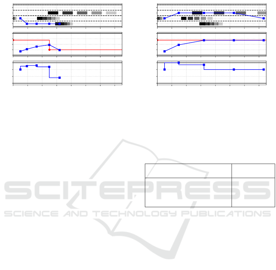
The ﬁrst situation is visualized in Figure 2. Here,

the simulated environment is a road section with four

lanes that are separated by dashed lane markings.

Implementation of Trajectory Planning for Automated Driving Systems using Constraint Logic Programming

415

−1

0.8

0.5

0.2

0.0

Lane advice:

v[ms

−1

]

min

max

0 20 40 60 80 100 120 140

[m]

−4

−2

a[m

−1

]

min

max

Figure 2: Resulting trajectory (blue) calculated by CLPTP

for a simulated trafﬁc situation consisting of 4 lanes, 4 other

dynamic objects with predicted movements (dark rectan-

gles) and 2 speed limits (red). Planning has been queried

for the discrete time instances 2 s, 4 s, 6 s and 8 s. At t = 0s,

the vehicle is in initial conﬁguration.

Hence, lane changes are allowed. Two speed limits

exist at s

= 0m and s

= 50m, respectively. Further-

more, there are four dynamic objects in addition to

the ego vehicle moving with different velocities. A

simple object prediction assuming objects to continue

on their current lane with their current velocity is ap-

plied for ease of demonstration. Predicted object po-

sitions are visualized for the discrete time instances

2 s, 4 s, 6 s and 8 s, for which planning is executed.

At t = 0 s, the vehicle is in initial conﬁguration. Val-

ues for strategic lane advice and important parameters

such as v

max

etc. are given in Figure 2 as well.

It can be seen that many requirements mentioned

in the previous section are fulﬁlled: Predictions of

other objects are considered. Strategic advice is taken

into account by a lane change. In general, velocity is

planned as high as possible. The second speed limit

results in an appropriate deceleration, but note that the

implementation in Listing 4 allows the vehicle to have

a velocity too high for the duration of one transition.

This could be adapted by an additional constraint for

the variable representing the velocity of the previous

conﬁguration.

The second situation is visualized in Figure 3. It

is similar to the ﬁrst situation but with the second

speed limit removed. Here, trajectory planning has

been queried for the time instances 3 s, 6 s, 9 s and 12 s

so that an overtaking maneuver can be demonstrated.

Due to the low velocity of the objects on the two

rightmost lanes, the results show that it is favourable

to change to the second leftmost lane despite its low

strategic advice in order to obtain a higher velocity.

This planning behaviour can of course be inﬂuenced

by the design of the costs that have been discussed in

−1

0.8

0.5

0.2

0.0

Lane advice:

v[ms

−1

]

min

max

0 20 40 60 80 100 120 140

[m]

−4

−2

a[m

−1

]

min

max

Figure 3: Resulting trajectory (blue) calculated by CLPTP

for a simulated trafﬁc situation consisting of 4 lanes, 4 other

dynamic objects with predicted movements (dark rectan-

gles) and 1 speed limit (red). Planning has been queried for

the discrete time instances 3 s, 6 s, 9 s and 12 s. At t = 0 s,

the vehicle is in initial conﬁguration.

Table 2: Execution time measurements for CLPTP (mea-

sured on a 2.5 GHz Intel



Core

i5-2450M with SICStus

Prolog 4.0.8).

Trafﬁc situation Execution

time

Situation 1 (Figure 2) 1427 ms

Situation 1 with a

max

= 1m

−1

360 ms

Situation 2 (Figure 3) 500 ms

Situation 2 with a

max

= 1m

−1

219 ms

Section 3.

Execution Time. Due to the dynamic environment

of real world automated vehicles, trajectories must be

planned cyclically at a high enough rate to account for

any changes in the environment. Thus execution time

is a critical characteristic for any trajectory planning

program.

Table 2 gives a summary of execution time mea-

surements for CLPTP. The results show that the com-

putational cost of our implementation is too high for

real world vehicles, where typical planning frequen-

cies lie in the range of 10 Hz to 20 Hz. However,

this does not mean that Prolog or CLP in general is

inappropriate for solving the problem of trajectory

planning, as the performance of the system is solely

determined by the labeling, search and optimization

algorithms of the underlying interpreter. For exam-

ple, if it is more appropriate to conduct a breadth-ﬁrst

search (as the A* algorithm does) instead of a depth-

ﬁrst search, this can be implemented in the interpreter

without modifying the declarative code it executes.

This inherent separation of logic describing a prob-

lem to solve and operational control ﬂow can be seen

as one of the advantages of CLP over other, e.g. im-

ICAART 2019 - 11th International Conference on Agents and Artiﬁcial Intelligence

416

perative, programming paradigms when solving com-

plex problems.

The results in Table 2 also illustrate the heavy in-

ﬂuence the size of the quantized conﬁguration space

has on execution time performance. Due to the safety-

criticality of trajectory planning, this is a signiﬁcant

issue because international standards for functional

safety such as ISO 26262 demand worst-case execu-

tion time estimations for any safety-relevant software.

Worst-case execution times can only be estimated for

trajectory planning programs if upper bounds are ap-

plied for the number of lanes, dynamic objects, speed

limits etc. The automated driving system system

can then only be applied safely in trafﬁc situations

not exceeding the estimated limits and mechanisms

(e.g. handover to a human driver) ensuring functional

safety in unexpectedly complex situations must be

implemented.

Veriﬁability. Two important methods are commonly

used to verify or validate safety-critical systems (ISO,

2011): On the one hand, there are formal techniques

like theorem proving. On the other hand, there is

systematic testing. Both methods can proﬁt from the

characteristics of CLP.

Theorem proving is based on ﬁrst-order

logic (Ray, 2010). Assertions on a program are

proved using logic inference. Since constraint logic

programs are also based on ﬁrst-order logic, the

application of theorem proving to them is more

straightforward compared to imperative programs.

To demonstrate how CLP supports writing sys-

tematic tests efﬁciently, Listing 6 outlines a simple

test case for CLPTP. The interpreter executing the

test case infers whether the lateral coordinate D of the

ﬁrst vehicle conﬁguration of any trajectory calculated

by CLPTP lies within certain lane boundaries.

Listing 6: Test case for CLPTP checking that lateral coordi-

nates lie within lane boundaries. Partial data structures and

double negation are used to make the test case as generic as

possible. The predeﬁned predicate assertz/1 is used to set

up a test scenario. fd_dom/2 is used to check the domain of

the constraint variable D.

:- ass e r t z ( o b j e c t (_ , _ , _ , _ , _ , _ )) .

:- ass e r t z ( s p eed _ l i mit ( _ , _ ) ) .

:- ass e r t z ( r igh t _ bou n d ar y (_ , -1) ) .

:- ass e r t z ( l eft _ b oun d a ry ( _ , 2) ).

:- \+( \ + ( ( tr a j e ctor y ([ _] , _ , [ conf (_ , D ,

_ ,_ , _) ] , _ ) , fd _ d o m (D , -1..2) ) ) ).

Note that the double negation used in the last di-

rective of Listing 6 is the usual Prolog method to

prove a test goal for all possible solutions and ensure

that variable bindings (in this case D) are unchanged

after executing the test goal. This test case example

uses the clause database of the interpreter for deﬁning

a test scenario and shows how partial data structures

allow generic tests. The test scenario in Listing 6 is

generic in so far that it includes trafﬁc situations with

arbitrary objects and speed limits by asserting facts

for the predicates object/6 and speed_limit/2 that

unify with any query. Thereby the independence of

staying within lane boundaries on the one side and

speed limits and objects on the other side is shown. In

other languages, multiple concrete test cases would

be needed to achieve an equivalent test coverage.

5 CONCLUSIONS AND FURTHER

WORK

The implementation of a general trajectory planning

module presented in this paper shows that CLP re-

duces the complexity of implementing a software

solving the problem of trajectory planning. Although

several simpliﬁcations have been applied for the ease

of demonstration, compared to imperative program-

ming languages, the translation of requirements and

constraints of the planning problem into program

code is more straightforward and easier to accomplish

for domain experts. Less operational details in the

code and the abstract, declarative way of specifying

knowledge about a problem as program code make

CLP a promising technology for the implementation

of software solving complex planning problems in au-

tomated driving systems. Compared to approaches

based on neural networks, well-known veriﬁcation

methods demanded by standards such as ISO 26262

can be applied more easily.

The execution time evaluation presented in Sec-

tion 4 shows that algorithms for constraint solving

and optimization currently available in interpreters of

CLP languages such as SICStus Prolog are not capa-

ble of fulﬁlling the performance requirements of auto-

mated driving systems in real world situations. How-

ever, the underlying algorithms of interpreters could

be adapted and improved without having to modify

the declarative code describing the problem to solve.

Future work should include an investigation on

how to improve execution time performance, e.g. by

using parallel implementations of constraint solving

and optimization algorithms. If execution time can

be reduced considerably, the approach of this paper

could be applied to implement not just general, but

also detailed trajectory planning. Smaller quantiza-

tion step sizes, high-dimensional conﬁguration spaces

and more accurate vehicle models could be used.

Implementation of Trajectory Planning for Automated Driving Systems using Constraint Logic Programming

417

REFERENCES

Apt, K. R. and Wallace, M. (2006). Constraint Logic Pro-

gramming Using ECLiPSe. Cambridge University

Press, Cambridge.

Arbib, J. and Seba, T. (2017). Rethinking Transporta-

tion 2020-2030: The Disruption of Transportation

and the Collapse of the Internal-Combustion Ve-

hicle and Oil Industries. Retrieved August 30,

2018, from https://www.rethinkx.com/s/RethinkX-

Report 051517.pdf.

Bauchau, O. A., editor (2011). Flexible Multibody Dynam-

ics. Solid Mechanics and Its Applications. Springer

Netherlands, Dordrecht.

Behere, S. and T

orngren, M. (2015). A Functional Archi-

tecture for Autonomous Driving. In Kruchten, P., Da-

jsuren, Y., Altinger, H., and Staron, M., editors, Pro-

ceedings of the First International Workshop on Auto-

motive Software Architecture - WASA ’15, pages 3–10,

New York, New York, USA. ACM Press.

Biran, O. and Cotton, C. (2017). Explanation and

Justiﬁcation in Machine Learning: A Survey.

In IJCAI-17 Workshop on Explainable AI (XAI)

Proceedings, pages 8–13. Retrieved December

3, 2018, from http://www.intelligentrobots.org/ﬁles/

IJCAI2017/IJCAI-17 XAI WS Proceedings.pdf.

Bojarski, M., Yeres, P., Choromanska, A., Choromanski,

K., Firner, B., Jackel, L. D., and Muller, U. (2017).

Explaining How a Deep Neural Network Trained

with End-to-End Learning Steers a Car. CoRR,

abs/1704.07911.

Carlsson, M. (2009). SICStus Prolog User’s Manual:

Release 4.0.8. Retrieved January 21, 2018, from

http://sicstus.sics.se/sicstus/docs/4.0.8/pdf/sicstus.pdf.

Carlsson, M. and Mildner, P. (2012). SICStus Prolog – The

ﬁrst 25 years. Theory and Practice of Logic Program-

ming, 12(1-2):35–66.

Diaz, D. (2001). Design and Implementation of the GNU

Prolog System. Journal of Functional and Logic Pro-

gramming, 2001(6).

Diaz, D., Abreu, S., and Codognet, P. (2012). On the im-

plementation of GNU Prolog. Theory and Practice of

Logic Programming, 12(1-2):253–282.

Dubey, A. D., Mishra, R. B., and Jha, A. K. (2013). Path

Planning of Mobile Robot using Reinforcement Based

Artiﬁcial Neural Network. Int. J. of Advances in En-

gineering & Technology, 6(2):780–788.

Grigorescu, S. M., Glaab, M., and Roßbach, A. (2017).

From logistic regression to self-driving cars:

Chances and challenges of using machine learning

for highly automated driving. Retrieved June 6,

2018, from https://d23rjziej2pu9i.cloudfront.net/wp-

content/uploads/2017/04/12081251/EB

TechPaper

From logistic regression to self driving cars.pdf.

Gu, T. and Dolan, J. M. (2012). On-Road Motion Planning

for Autonomous Vehicles. In Su, C.-Y., Rakheja, S.,

and Liu, H., editors, Intelligent robotics and applica-

tions, volume 7508 of LNAI, pages 588–597. Springer,

Berlin.

Hart, P., Nilsson, N., and Raphael, B. (1968). A Formal Ba-

sis for the Heuristic Determination of Minimum Cost

Paths. IEEE Transactions on Systems Science and Cy-

bernetics, 4(2):100–107.

ISO (2011). International Standard ISO 26262-6:2011(E):

Road Vehicles - Functional Safety - Part 6: Product

development at the software level.

ITF (2017). ITF Transport Statistics. OECD Publishing.

Kelly, A. and Nagy, B. (2016). Reactive Nonholonomic

Trajectory Generation via Parametric Optimal Con-

trol. The International Journal of Robotics Research,

22(7-8):583–601.

Lever, J. and Richards, B. (1994). parcPlan: A planning

architecture with parallel actions, resources and con-

straints. In Ra

s, Z. W., editor, Methodologies for intel-

ligent systems, volume 869 of LNAI, pages 213–222.

Springer, Berlin.

McNaughton, M. (2011). Parallel Algorithms for Real-time

Motion Planning. PhD thesis, Carnegie Mellon Uni-

versity, Pittsburgh, PA.

Paden, B., Cap, M., Yong, S. Z., Yershov, D., and Frazzoli,

E. (2016). A Survey of Motion Planning and Control

Techniques for Self-Driving Urban Vehicles. IEEE

Transactions on Intelligent Vehicles, 1(1):33–55.

Piaggio, M. and Sgorbissa, A. (2000). Real-Time Mo-

tion Planning in Autonomous Vehicles: A Hybrid Ap-

proach. In Goos, G., Hartmanis, J., van Leeuwen,

J., Lamma, E., and Mello, P., editors, AI*IA 99:

Advances in Artiﬁcial Intelligence, volume 1792 of

LNCS, pages 368–378. Springer, Berlin.

Rathgeber, C. (2016). Trajektorienplanung und -

folgeregelung f

ur assistiertes bis hochautomatisiertes

Fahren. PhD thesis, TU Berlin.

Ray, S. (2010). Scalable Techniques for Formal Veriﬁca-

tion. Springer US, Boston, MA.

Werling, M. (2011). Ein neues Konzept f

ur die Tra-

jektoriengenerierung und -stabilisierung in zeitkritis-

chen Verkehrsszenarien, volume 34 of Schriftenreihe

des Instituts f

ur Angewandte Informatik - Automa-

tisierungstechnik, Universit

at Karlsruhe (TH). KIT

Scientiﬁc Publishing, Karlsruhe.

Werling, M., Ziegler, J., Kammel, S., and Thrun, S. (2010).

Optimal trajectory generation for dynamic street sce-

narios in a Fren

et Frame. In 2010 IEEE International

Conference on Robotics and Automation, pages 987–

993. IEEE.

Wielemaker, J., Schrijvers, T., Triska, M., and Lager, T.

(2012). SWI-Prolog. Theory and Practice of Logic

Programming, 12(1-2):67–96.

Ziegler, J. and Stiller, C. (2009). Spatiotemporal state lat-

tices for fast trajectory planning in dynamic on-road

driving scenarios. In 2009 IEEE/RSJ International

Conference on Intelligent Robots and Systems, pages

1879–1884, Piscataway, NJ. IEEE.

Zuo, B., Chen, J., Wang, L., and Wang, Y. (2014). A rein-

forcement learning based robotic navigation system.

In 2014 IEEE Int. Conf. on Systems, Man, and Cyber-

netics (SMC), pages 3452–3457. IEEE.

ICAART 2019 - 11th International Conference on Agents and Artiﬁcial Intelligence

418