Asynchronous Price Stabilization Model in Networks
Jun Kiniwa
1
, Kensaku Kikuta
1
and Hiroaki Sandoh
2
1
Department of Applied Economics, University of Hyogo, 8-2-1 Gakuen-nishi, Nishi, Kobe, 651-2197, Japan
2
School of Policy Studies, Kwansei Gakuin University, 2-1 Gakuen, Sanda, Hyogo, Japan
Keywords:
Multiagent Model, Fisher’s Quantity Equation, Velocity of Money, Asynchronous System.
Abstract:
We consider a multiagent network model consisting of nodes and edges as cities and their links to neighbors,
respectively. Each network node has an agent and priced goods and the agent can buy or sell goods in the
neighborhood. Though every node may not have an equal price, we can show the prices will reach an equi-
librium by iterating buy and sell operations. We introduce a framework of protocols in which each buying
agent makes a bid to the lowest priced goods in the neighborhood; and each selling agent selects the high-
est bid (if any). So far, we have just considered such a model in a synchronous environment. We, however,
cannot represent the velocity of circulation of money in the synchronous system. In other words, we cannot
distinguish the different speed of money movement if every operation is synchronized. Thus, we develop an
asynchronous model which enables us to generalize the theory of price stabilization in networks. Finally, we
execute simulation experiments and investigate the influence of network features on the velocity of money.
1 INTRODUCTION
Background. Conventionally, the topic of price de-
termination has been discussed from microeconomics
approach(N.G.Mankiw, 2018). In the presence of ap-
propriate supply and demand curves, if the price is
higher (resp. lower) than an equilibrium, there is ex-
cess supply (resp. excess demand) and thus the price
moves to the equilibrium. At the equilibrium price,
the quantity of goods sought by consumers is equal to
the quantity of goods supplied by producers. Neither
consumers nor producers have incentive to change the
price /quantity at the equilibrium.
In contrast, we considered a multiagent network
model (J.Kiniwa and K.Kikuta, 2011a; J.Kiniwa and
K.Kikuta, 2011b; J.Kiniwa et al., 2017b), in which
each agent repeatedly makes auctions and the price of
goods is eventually determined. Our network model
consists of nodes and edges as cities and their links to
neighbors, respectively. Each node contains an agent
which represents people living in the city. Agents
who want to buy goods make bids to the lowest-priced
neighboring node, if any. Then, agents who want to
sell the goods accept the highest bid. We have shown
the reason of price determination by using the idea
of self-stabilization in distributed systems(S.Dolev,
2000). From any initial state, self-stabilizing algo-
rithms eventually lead to a legitimate state without
any aid of external actions. Such a self-stabilization
resembles the price determination, where the price
reaches an equilibrium without external operations.
Motivation. Our first work was motivated by an
intuition that simulating trades between agents may
stabilize the price instead of the supply-demand the-
ory. We developed a trading model using auctions
in which prices converge to a unique one(J.Kiniwa
and K.Kikuta, 2011a; J.Kiniwa and K.Kikuta, 2011b).
We, however, were not able to explain why such a
unique price is determined. After that, we assumed a
relation p
i
= m
i
/q
i
between the price p
i
, goods q
i
and
money m
i
at each node i, and each agent exchanges
money and goods. Then, it enables us to estimate an
equilibrium price P
e
= M/T, where M =
∑
i
m
i
and
T =
∑
i
q
i
(J.Kiniwa et al., 2017b). Further, we de-
veloped a method of expected optimal bidding and
derived the difference between two presenting proto-
cols (J.Kiniwa et al., 2017a). We, however, were not
able to distinguish whether or not the convergence is
fast because the velocity of money is always constant.
Problem. Irving Fisher’s claim, MV
m
= P
e
T, has
been accepted as the quantity theory of money, where
V
m
is the velocity of money. The correctness of our
synchronous model was guaranteed by Fisher’s quan-
tity equation with V
m
= 1. However, since the equa-
tion describes an arbitrary velocityV
m
, there must ex-
ist some method which corresponds to such an exten-
Kiniwa, J., Kikuta, K. and Sandoh, H.
Asynchronous Price Stabilization Model in Networks.
DOI: 10.5220/0007306701210128
In Proceedings of the 11th International Conference on Agents and Artificial Intelligence (ICAART 2019), pages 121-128
ISBN: 978-989-758-350-6
Copyright
c
 2019 by SCITEPRESS – Science and Technology Publications, Lda. All rights reserved
121

sion. So, our first issue was how to extend the model
to an arbitrary velocity V
m
. If it were possible, our
network model could be guaranteed by the Fisher’s
quantity equation in general. Next, our second issue
was how to compute the velocity of money. If it were
possible, the velocity of money could be explicitly de-
rived. Then, we could know whether the velocity of
money is different in several network topologies and
protocols.
Solution. For the first issue, we develop an asyn-
chronous price stabilization model in order to express
an arbitrary velocity V
m
of money. We can use the
concept of asynchronous round or simply round, an
appropriate interval, and define the velocity as the ba-
sis of the slowest agent: In a round, the slowest agent
trades only once, while the others do at least once.
Then, the money payed by the slowest agent moves
only distance 1, while the other money moves farther.
So, the different speed between money gives the con-
cept of velocity.
For the second issue, we consider a variable
flow
i
of money used at each node i. The sum of
flow
i
through the network means the total quantity of
money that was repeatedly used in a round. We con-
sider the velocity of money as the sum of flow
i
divided
by the amount of money supply. Since the moneysup-
ply is constant, the velocity of money becomes large
if the sum of flow
i
grows.
Related Work. The classical theory of price
determination in microeconomics is introduced in
(N.G.Mankiw, 2018). In contrast to the conven-
tional work, we review the theory from a multiagent
viewpoint. There exist a large body of literature on
social economic networks (J.Benhabib et al., 2010)
containing a network formation game (M.O.Jackson
and A.Wolinsky, 1996) and a buyer-seller net-
work (M.O.Jackson and A.Watts, 2010; R.Kranton
and D.Minehart, 2001). The network formation game
considers the choice of relationships between agents,
and the buyer-seller network considers the competi-
tion and exchange in bipartite networks (E.Even-Dar
et al., 2007; R.Kranton and D.Minehart, 2001). Un-
like their interest in maximizing economic surplus,
our work focuses on price stabilization. Auction the-
ory has been comprehensively studied in (V.Krishna,
2002). Our protocol in Section2.2 may be consid-
ered as a consensus algorithm. The consensus al-
gorithm is described in (N.A.Lynch, 1996), and its
self-stabilizing version is described in (S.Dolev et al.,
2010). However, their work cannot be categorized
as economics. Asynchronous systems have been ex-
tensively discussed in the area of distributed algo-
rithms(N.A.Lynch, 1996). This is because most of
the distributed algorithms must work in such an envi-
ronment. Thus the multiagent system should be de-
scribed as an asynchronous system.
Our previous work (J.Kiniwa and K.Kikuta,
2011a) considers a naiveprotocol in which each buyer
makes a bid with an appropriate rate to a seller. Then,
(J.Kiniwa and K.Kikuta, 2011b) and (J.Kiniwa et al.,
2017b) analyze the best bidding price for a con-
stant number of bidders, and (J.Kiniwa et al., 2017b)
assumes the price is determined by the amount of
money and goods.
Contributions. We propose an asynchronous price
stabilization model in this paper. We consider the
asynchronous system is not only as an extension of
the synchronous system but also as a method of mea-
suring the velocity of money. We define the velocity
of money as the total spent money divided by the total
supplied money in a round. To compare the velocity
of money, we execute simulation experiments for two
networks and three protocols. Then we obtain some
reasonable results, that is, the velocity of money is
fast if there is a lot of payment.
We organize the rest of this paper as follows. Sec-
tion2 states our model and protocols. Section 3 dis-
cusses how we can represent the velocity of money.
Section4 shows some results of simulation experi-
ments for several networks and protocols. Finally,
Section5 concludes the paper.
2 MODEL
Here we describe our model consisting of a network
in section 2.1, a protocol design in section 2.2, and
the expected number of bidders in section 2.3.
2.1 Network
Our system can be represented by a connected net-
work G = (V,E), consisting of a set of nodes V and
edges E, where the nodes represent cities and a pair of
neighboringnodes is linked by an edge. Let N
i
be a set
of neighboring nodes of i ∈ V, and let N
+
i
= N
i
∪ {i}.
We assume that each node i ∈ V has a good of one
single type and their initial price may be distinct. Let
p
i
be the price of the goods at node i. Each node i ∈ V
has exactly one representative agent a
i
who always
stays at i and can buy goods in the neighborhood N
i
.
Each agent a
i
has money m
i
and the quantity q
i
of
goods. The price p
i
is determined by the relation be-
tween the quantity of goods and the buying power,
called a supply-demand balance. So we simply as-
sume two properties at each node. First, the price
is proportional to the amount of money for constant
goods. Second, the price is inversely proportional to
ICAART 2019 - 11th International Conference on Agents and Artificial Intelligence
122

the amount of goods for constant money. That is,
p
i
=
m
i
q
i
. (⋆)
If the total amount of goods q
i
are sold at each node
i, then the total trade at i is equal to q
i
. By summing
up q
i
for every node, we can verify the correctness
of these assumptions by the Fisher’s quantity equa-
tion(N.G.Mankiw, 2018).
The buy operation is executed as follows. Each
agent a
i
assigns a value v
j
i
to the goods of any neigh-
boring node j ∈ N
i
, where the value means the max-
imum amount an agent is willing to pay. Agent a
i
compares its own goods price p
i
with the neighboring
price p
j
. If the cheapest price in N
i
is p
j
(< p
i
), agent
a
i
wants to buy it and makes a bid b
j
i
to node j. We
consider v
j
i
= p
i
for any j ∈ N
i
because he can buy it
at price p
i
in his node (V.Krishna, 2002).
The sell operation is executed as follows. After
accepting bids, agent a
j
contracts with a
i
∈ N
j
, who
made the highest bid b
j
i
at some appropriate time,
called a contract time. Agent a
j
passes a
i
goods, and
conversely agent a
i
passes a
j
money. Such trades are
repeated until the price p
j
becomes equal to p
i
caused
by the exchange of goods and money between them.
We do not take the carrying cost of goods into consid-
eration but focus on the change of prices. Each node
i ∈ V has a state Σ
i
represented by a tuple — the goods
and the money (q
i
,m
i
).
We assume an asynchronous model, that is, every
agent aperiodically executes operations, exchanges
messages, and knowsthe states of neighboringagents.
We call the state of all nodes a configuration. A
configuration is legitimate if every node has equally
priced goods. In the asynchronous system, there is no
bound on the rate of step-execution. However, it is
convenient to use the number of asynchronous rounds
or rounds in order to evaluate the system. The first
round in an execution E is the shortest prefix E
′
of
E such that each agent executes at least one step in
E
′
. Let E
′′
be the suffix of E that follows E
′
, that is,
E = E
′
E
′′
. The second round of E is the first round
of E
′′
, and so on. Intuitively, we can regard a round
as the time interval between the two operations of the
slowest agent.
2.2 Protocol Design
In this section, we first consider a protocol model,
called a first-price protocol (FirstPrice). In the pro-
tocol, each agent a
i
asynchronously makes a bid b
j
i
to
an agent a
j
∈ N
i
with the lowest price in the neighbor-
hood. However, all the bids to a
j
may not be submit-
ted yet when a
j
chooses the highest one. The follow-
ing assumption means that once a contract is made, it
is known to neighbors and a new submission of bid is
suppressed until the agents complete the trade.
Assumption 1. Once a buyer and a seller have made
a contract, they complete the trade until their prices
are balanced without interference. ⊓⊔
FirstPrice
1. Each agent a
i
makes a bid b
j
i
to node j ∈ N
i
which
has the lowest-priced goods in N
i
and less than p
i
.
2. At a contract time, the agent a
j
contracts with
the neighboring a
h
1
who has made the highest bid
max
h
1
∈N
j
b
j
h
1
at the time. The goods moves from
q
j
to q
h
1
and the money moves from m
h
1
to m
j
at
h
1
’s bidding price b
j
h
1
as long as p
h
1
> p
j
. The
new prices p
h
1
and p
j
after the exchange are de-
termined by the amount of money/goods.
3. If several agents make bids to node j with the
same highest price, agent a
j
makes deals with one
of them at random.
4. (priority rule:) If concurrent buy (b
k
j
to k ∈ N
j
)
and sell (b
j
h
from h ∈ N
j
) operations occur at agent
a
j
, he gives priority to the sell over the buy.
If 2 above is replaced by the following 2
′
, we call it
a second-price protocol (SecondPrice). Let agent a
h
2
have made the secondly highest bid to node j, called
a secondly bidder.
2
′
. At a contract time, the agent a
j
contracts with
the neighboring a
h
1
who has made the highest bid
max
h
1
∈N
j
b
j
h
1
at the time. The goods moves from
q
j
to q
h
1
and the money moves from m
h
1
to m
j
at
the secondly bidder a
h
2
’s bidding price b
j
h
2
as long
as p
h
1
> p
j
.
In summary, if buyer a
i
pays his bidding price to
seller a
j
, we call the protocol a first-price protocol.
In contrast, if buyer a
i
pays the secondly highest (i.e.,
other buyer’s) bidding price to seller a
j
, we call the
protocol a second-price protocol.
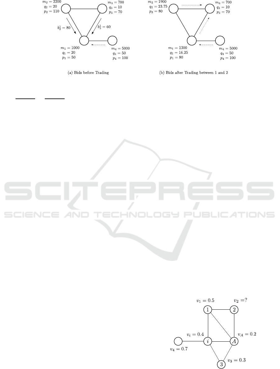
Example 1. Figure1 shows an example of our net-
work system consisting of 4 nodes V = {1,2,3,4}.
At first, the prices of goods are (p
1
, p
2
, p
3
, p
4
) =
(50,110,70,100) as shown in Figure1(a). Each
agent a
i
wants to buy the lowest-priced goods at
node j ∈ N
i
if its price is lower than p
i
, that is,
p
i
> min
j∈N
i
p
j
. Thus, both a
2
and a
3
make bids to
node 1. The action of a
4
, however, is too slow to
attend the a
1
’s contract time (The anticipated oper-
ation is depicted as a dotted arrow). Since agent
a
2
beats a
3
, agent a
2
makes a contract with agent
a
1
. Let x units be the number of a
2
’s buying goods.
Asynchronous Price Stabilization Model in Networks
123

1
2
3
4
1
2
3
4
Figure 1: An illustration of protocol FirstPrice (Intermediate bidding).
Since the prices of nodes 1 and 2 become equal, we
have
1000+80x
20−x
=
2200−80x
20+x
. This gives x = 3.75 and
hence q
1
= 20−x = 16.25, q
2
= 20+x = 23.75, m
1
=
1000+ 80x = 1300, and m
2
= 2200− 80x = 1900.
After the trade as above, the prices become
(p
1
, p
2
, p
3
, p
4
) = (80,80,70,100) as shown in Fig-
ure 1(b). Here, agents a
1
and a
2
can make bids to
node 3, and agent a
4
can make a bid to node 1. If b
1
4
and b
3
1
cuncurrently occur at node 1, agent a
1
gives
priority to b
1
4
and delays b
3
1
because of avoiding con-
fusion (see the “priority rule”). ⊓⊔
We concern about whether the prices of goods
eventually reach an equilibrium price even if they are
initially distinct. The following lemma states an asyn-
chronous issue.
Lemma 1. Even if there is a slow operating agent,
the protocols correctly work.
Proof. Suppose that there is a too slow operating
agent i and other agents operates much faster than i.
We have to consider two cases.
1. The removal of node i separates the network into
two or more components.
2. The removal of node i does not separate the net-
work.
Suppose the move of i, a pair of buy and sell opera-
tions of i, is slow enough to stabilize the price in each
component.
In the first case, let C
j
and C
k
be two components
of them and p
j
and p
k
be their prices, where p
j
< p
i
<
p
k
, respectively. Let diff
h
( j,k) the price difference
between p
j
and p
k
after the h-th move of i. After the
first move of agent i, some goods move from C
j
to i
and then from i to C
k
. Likewise, some money move
from i to C
j
and then from C
k
to i. Thus, diff
0
( j,k) >
diff
1
( j,k) holds. This can be inductively proved.
In the second case, only price p
i
is different from
others. Thus, the moves of i eventually stabilize the
price. ⊓⊔
In (J.Kiniwa and K.Kikuta, 2011b), we examined
a sufficient condition for price stabilization in First-
Price. Suppose that agents a
i
and a
j
make bids to
node h ∈ N
i
∩ N
j
. We say that bids have the same or-
der as values if v
h
i
≤ v
h
j
implies b
h
i
≤ b
h
j
for the goods
of node h. The following theorem further shows that
an additional condition leads to the price stabilization.
Theorem 1. (J.Kiniwa and K.Kikuta, 2011b) Sup-
pose bids keep the same order as values. If any
contract price lies between buyer’s price and seller’s
price, price stabilization occurs. ⊓⊔
2.3 Expected Number of Bidders
In our network model, each agent makes a bid to the
minimal priced node in the neighborhood. Since the
prices vary from time to time, the minimal priced
node also changes. So, we consider the expected
number of bidding nodes.
Assumption 2. We assume every agent can know the
maximum / minimum price, and we assume the value
v
i
is equal to the price p
i
at node i. The values are
uniformly distributed over (0, 1). ⊓⊔
Next, Assumption 3 is necessary for computing
expected number of bidders.
Assumption 3. Agent i knows any node u within dis-
tance 3 from i. ⊓⊔
4
Figure 2: Certain agent (node 3) vs. uncertain agent (node
2) for i with respect to A.
ICAART 2019 - 11th International Conference on Agents and Artificial Intelligence
124

Figure 2 illustrates an example in which node A
sells goods and some nodes in N
A
make bids to A. Let
v
u
(= p
u
) be the value of agent u, and the price p
u
for each u is not explicitly depicted. Suppose agent
i wants to make a bid to A. Since agent i is not ad-
jacent to agent 2, he does not know agent 2’s value,
however, knows the existence of node 2 and N
2
(by
Assumption3). Since agent 1 is adjacent to agent 2,
agent i does not know agent 1’s behavior. Thus the
uncertain decisions of agent 1 and agent 2 depend on
N
+
1
\N
i
= {2} and N
+
2
\N
i
= {2}, respectively. Fur-
ther notice the decision of agent 1 depends on agent
2’s value, that is, agent 1 makes a bid to A if v
2
> v
A
.
We say that such agent 1 is dependent on 2 with re-
spect to A. Agent i surely knows agent 3 makes a bid
to A because v
A
< v
3
. We call such agent 3 a certain
agent for i with respect to A. Let P(ρ
u
) (resp. P(σ
u
))
be the probability that agent u makes (resp. does not
make) a bid to A, and let k
u
be the number of |N
+
u
\N
i
|.
Thus, the probabilities that make bids to A are
(P(ρ
1
),P(ρ
2
),P(ρ
3
)) = ((1− v
A
)
k
1
,(1− v
A
)
k
2
,1)
= (0.8,0.8, 1),
where P(ρ
1
ρ
2
) = P(ρ
2
) and P(ρ
1
σ
2
) = P(σ
1
ρ
2
) = 0.
We consider probability P
i
( j) that there are j bidding
nodes to A when agent i makes a bid to A. Then, the
probability that four agents make bids to A is
P
i
(4) = P(ρ
i
ρ
1
ρ
2
ρ
3
) = P(ρ
i
ρ
2
ρ
3
) = 1· 0.8· 1.
The probability that three agents make bids to A is
P
i
(3) = P(ρ
i
ρ
1
σ
2
ρ
3
) + P(ρ
i
σ
1
ρ
2
ρ
3
) = 0.
The probability that two agents make bids to A is
P
i
(2) = P(ρ
i
σ
1
σ
2
ρ
3
) = P(ρ
i
σ
2
ρ
3
) = 1· 0.2· 1.
More formally, the probability that v
A
is the small-
est value in |N
+
u
\N
i
| is P(ρ
u
) = (1 − v
A
)
k
u
. Con-
versely, the probability that v
A
is not the smallest
value is P(σ
v
) = 1 − (1 − v
A
)
k
v
. For independent
agents u
s
and u
t
, we can represent
P
i
( j) =
∑
P(ρ
i
)=1



∏
1≤s≤ j
j+1≤t≤N
A
P(ρ
u
s
)P(σ
u
t
)



.
If k
u
= |N
+
u
\N
i
| = 0, agent i knows every neigh-
boring value of u, and thus understands whether agent
u makes a bid to A. Otherwise, agent i cannot know
some neighboring values of u, and thus estimates the
possibility of u’s bidding. We call such agent u an
uncertain agent for i with respect to A.
It is known that Bayesian-Nash equilibrium oc-
curs when each agent i makes a bid ( j− 1)/ j·v
i
when
there are j bidders(V.Krishna, 2002). We consider the
expectation of ( j − 1)/ j, called an expected rate. The
expected bidding rate, denoted by R
I
i
, of the Bayesian-
Nash equilibrium is
R
I
i
=
|N
A
|
∑
j=|C
A
i
|+1
j − 1
j
P
i
( j),
where C
A
i
be the set of certain bidders for i which
make bids to A. (J.Kiniwa et al., 2017a) has also
shown that the optimal bidding rate of our second-
price protocol is
R
II
i
= 1.
Thus, the optimal bidding price for FirstPrice and
SecondPrice is b
A
i
= R
I
i
v
i
and b
A
i
= v
i
, respectively.
Theorem 2. (J.Kiniwa et al., 2017a) In arbitrary
networks, price stabilization is guaranteed by our
second-price protocol. In contrast, it is not always
guaranteed by our first-price protocol. ⊓⊔
We call the first-price protocol (resp. second-price
protocol) with its optimal bidding rate FirstOptBid
(resp. SecondOptBid). Since the price stabilization
is not always guaranteed by the FirstOptBid in any
network(J.Kiniwa et al., 2017a), we introduce the fol-
lowing alternative protocols instead of FirstOptBid,
• Intermediate bidding (with first-price) protocol, and
• Pseudo first-price (with optimal bidding) protocol.
In the former protocol, each buyer makes an inter-
mediate bid between the buyer’s price and the seller’s
price, and pays his bidding price, as illustrated in Fig-
ure 1. In the latter protocol, the highest priced agent
makes an optimal bid and always wins his contract
with a seller. Though some agent may not follow the
auction rule, we just consider it from the viewpoint of
circulation of money. The price stabilization is guar-
anteed by both methods.
3 VELOCITY OF MONEY
In the synchronousmodel(J.Kiniwa et al., 2017b), we
already have the following result.
Theorem 3. (J.Kiniwa et al., 2017b) Let T be the to-
tal volume of transactions, interpreted as the quantity
of goods, and let M be the total amount of money. In
any synchronous system, the equilibrium price P
e
in a
connected network G is presented by
P
e
=
M
T
.
⊓⊔
Notice that this equality coincides with Fisher’s
quantity equation MV
m
= P
e
T when V
m
= 1.
Asynchronous Price Stabilization Model in Networks
125

To extend this to general V
m
, we have to consider
an asynchronous system in which every operation oc-
curs at any time. The velocity of money is defined as
the mean distance money is passed from one holder
to the next in a round.
Let flow
i
be a variable which represents cumula-
tively paid money at node i. The velocity of money is
obtained as in the following theorem.
Theorem 4. Suppose that each node i has paid money
of flow
i
in a round. Then, the velocity V
m
of money is
V
m
=
∑
i
flow
i
M
.
Proof. In the Fisher’s equation MV
m
= P
e
T, the right-
hand side P
e
T means the total amount of selling goods
in the system. It is equal to the total amount of paid
money in the system. Thus, we can measure it by
using the variable flow
i
for every node i ∈ V. Then we
have P
e
T =
∑
i
flow
i
. Therefore, the theorem follows.
⊓⊔
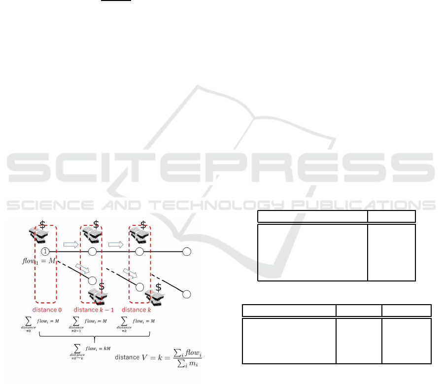
Figure 3 illustrates the idea of velocity of money.
For simplicity, suppose agent 1 holds money M at
time 0. Then, it passes through several nodes and each
agent i records his spent money in flow
i
. At the end
of the round, suppose all the money M reaches nodes
distance k from node 1. Then, the total sum of flow
i
consists of the sums of them with respect to distance
0,1,...,k. Thus the distance k during one round, the
velocity of money, is derived as in Theorem4.
Figure 3: Distance of Money Traveling.
4 SIMULATION
In this section, we execute simulation experiments for
the protocols above in path and grid networks. We in-
vestigate the influence of the network topologies and
other aspects on the velocity of money.
Next, we consider the following three issues in
two kinds of networks, a path and a grid. If we ex-
ecute (a) intermediate bidding protocol, (b) pseudo
first-price protocol, and (c) SecondOptBid, we inves-
tigate how
[1] the number of nodes,
[2] the number of money-injection nodes, and
[3] the rate of concurrency
have great influence on the velocity of money. More
precisely, [1] we increase/decrease the number of
nodes, [2] we add much money at some selected
nodes, called money-injection nodes, and change the
number of them, and [3] we change the number of
concurrently trading agents.
Table 1 shows the constants used in our exper-
iments. We repeat the experiment up to 50 trials,
where a trial ends with an equilibrium, and obtain
mean results. Initially, each node has money 100
units, and has goods between 50 and 100 units at ran-
dom. Then, the equation (⋆) determines the price for
each node. The total injection of money is 30,000
units. Table 2 shows the parameters used in our ex-
periments. It has the third column named “standard”
which means a constant value if another parameter is
being varied. For example, the number of nodes is
300 when we vary the number of injection nodes from
1 to 10, or when we vary the rate of concurrencyfrom
0.1 to 0.9, and so on.
Table 1: Constants.
Meaning Value
Number of Trials 50
Iteration 500
Money per Node 100
Goods per Node [50, 100]
Total Injection of Money 30,000
Table 2: Parameters.
Meaning Value Standard
Number of Nodes 50—500 300
Number of Money
-injection Nodes 1—10 1
Rate of Concurrency 0.1—0.9 0.5
4.1 Number of Nodes
Figures4 and 5 show how the number of nodes has
influence on the velocity of money in two networks.
All the curves increase as the number of nodes grows
because there may be some extremely slow agents in
large population. In the path, since almost all nodes
have two degrees, not so many conflicts of bidding
occur. Thus the payment of two equilibrium bidding
ICAART 2019 - 11th International Conference on Agents and Artificial Intelligence
126

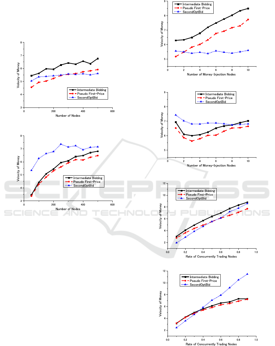
protocols is low and that of the intermediate bidding
protocol is high. In the grid, the payment of the
second-price protocol is higher than others because
each bidder i makes a bid b
j
i
= v
j
i
to j ∈ N
i
and pays
the second highest bid.
Figure 4: Varying Number of Nodes in Path.
Figure 5: Varying Number of Nodes in Grid.
4.2 Money-injection Nodes
Figures6 and 7 show how the number of money-
injection nodes has influence on the velocity of money
in two networks. In the path, since many number of
money-injection nodes grow the spread of money in
intermediate pseudo first-price protocols, the velocity
of money becomes high. On the other hand, the influ-
ence of the second-price protocol is not outstanding.
This is because the payment from a money-injection
node would be equal to the bidding price of its neigh-
boring nodes. And then, the payment would be low
in the second-price protocol. Thus, the velocity of
money in the second-price protocol is slow. In the
grid, the tendency of the former two protocols looks
alike.
4.3 Concurrently Trading Nodes
Figures8 and 9 show how the number of concurrently
trading nodes has influence on the velocity of money
Figure 6: Varying Money-Injection Nodes in Path.
Figure 7: Varying Money-Injection Nodes in Grid.
Figure 8: Varying Concurrently Trading Nodes in Path.
Figure 9: Varying Concurrently Trading Nodes in Grid.
in two networks.In the path, since the conflicts of bid-
ding do not occur so often, the curves grow according
as the rate of concurrently trading nodes. In the grid,
Asynchronous Price Stabilization Model in Networks
127

since winner’s payment of the second-price protocol
is higher than others, the velocity of money is fast.
5 CONCLUSION
In this paper we extended our synchronous model
for the price stabilization to an asynchronous system.
Then we have obtained the following two advantages:
• we can consider a general model which is close to
an actual system, and
• we can explain the velocity of money in Fisher’s
quantity equation.
First, we described how to express the velocity of
money in Section3. Then, we executed simulation
experiments and revealed several features of the ve-
locity of money in a path and a grid in Section4.
The velocity of money for the second-price proto-
col is faster than that for the first-price protocol. Such
a property is remarkable in grid networks rather than
in path networks. This is because the second-price
protocol accepts higher bidding price for many bid-
ders, and then the amount of trade grows at an inter-
val.
Our future work includes developing a practical
stabilization model, for example, on-line shopping,
and other protocols.
ACKNOWLEDGEMENTS
This work was supported by JSPS KAKENHI Grant
Number ((C)17K01281).
REFERENCES
E.Even-Dar, M.Kearns, and S.Suri (2007). A network for-
mation game for bipartite exchange economies. In
Proceedings of the 18th ACM-SIAM Simposium on
Discrete Algorithms (SODA 2007), pages 697–706.
J.Benhabib, M.O.Jackson, and (ed.), A. (2010). Handbook
of social economics, volume 1a. North Holland, Am-
sterdam, 1st edition.
J.Kiniwa and K.Kikuta (2011a). A network model for
price stabilization. In Proceedings of the 3rd Inter-
national Conference on Agents and Artificial Intelli-
gence (ICAART), pages 394–397.
J.Kiniwa and K.Kikuta (2011b). Price stabilization in net-
works — what is an appropriate model ? In 13th In-
ternational Symposium, SSS2011: LNCS 6976, pages
283–295. Springer.
J.Kiniwa, K.Kikuta, and H.Sandoh (2017a). Equilibrium
bidding protocols for price stabilization in networks.
In 4th International Conference on Behavioral, Eco-
nomic, and Socio-Cultural Computing, BESC2017,
pages 1–6.
J.Kiniwa, K.Kikuta, and H.Sandoh (2017b). A price stabi-
lization model in networks. Journal of the Operations
Research Society of Japan, 60(4):479–495.
M.O.Jackson and A.Watts (2010). Social games: matching
and the play of finitely repeated games. Games and
Economic Behavior, 70:170–191.
M.O.Jackson and A.Wolinsky (1996). A strategic model of
social and economic networks. Journal of Economic
Theory, pages 44–74.
N.A.Lynch (1996). Distributed Algorithms. Morgan Kauf-
mann Publishers, San Francisco, California, 1st edi-
tion.
N.G.Mankiw (2018). Principles of economics. Cengage
Learning, Boston, Massachusetts, 8th edition.
R.Kranton and D.Minehart (2001). Theory of buyer-seller
networks. American Economic Review, 91(3):485–
508.
S.Dolev (2000). Self-stabilization. The MIT Press, Cam-
bridge, Massachusetts, 1st edition.
S.Dolev, R.I.Kat, and E.M.Schiller (2010). When consen-
sus meets self-stabilization. Journal of Computer and
System Sciences, 76:884–900.
V.Krishna (2002). Auction theory. Academic Press, San
Diego, 1st edition.
ICAART 2019 - 11th International Conference on Agents and Artificial Intelligence
128