
Robust Person Identification based on DTW Distance of Multiple-Joint
Gait Pattern
Takafumi Mori
1
and Hiroaki Kikuchi
2
1
Graduate School of Advanced Mathematical Sciences, Meiji University, 164-8525, Japan
2
School of Interdisciplinary Mathematical Science, Meiji University, 164-8525, Japan
Keywords:
Gait, Biometrics, DTW, Person Identification.
Abstract:
Gait information can be used to identify and track persons. This work proposes a new gait identification
method aggregating multiple features observed by a motion capture sensor and evaluates the robustness against
obstacles in walking. The simplest gait identification is to use gait statistics, but these are not a significant
feature with regard to identifying people accurately. Hence, in this work, we use the dynamic time warping
(DTW) algorithm to calculate distances of gait sequences. DTW is a pattern-matching algorithm mainly used
in speech recognition. It can compare two sets of time series data, even when they have different lengths. We
also propose an optimal feature integration method for DTW distances. For evaluating the proposed method,
we developed a prototype system and calculated the equal error rate (EER) using 31 subjects. As a result,
we clarified that the EER of the proposed method is 0.036 for normal walking, and that it is robust to some
obstacles in walking.
1 INTRODUCTION
Gait information can be used to identify and track per-
sons because there are several advantages to using a
person’s gait features. For example, the features can
be observed by outside sensors, can easily be aggre-
gated for multiple features, and target cooperation is
unnecessary. The consumer market industry has a
strong demand for automatically tracking persons and
for big-data analysis of the behavior of a large number
of customers in a store. Gait information can be used
to track customers without their consent to be tracked.
It is important to pay attention to economical cost of
security systems in modern applications (Sklavos and
Souras, 2006).
The simplest form of gait identification is to use
statistics of human joint distance. For example, we
identify people by an average distance between hands.
However, statistics are not suitable for doing so be-
cause of the following difficulties:
• The dynamic distance between hands is not stable
and changes frequently, even in the same person.
• The static distance between joints does not have
a high enough resolution to distinguish between
individuals.
In order to solve the issues with regard to gait
identification, we used the dynamic time warping
(DTW) (Berndt and Clifford, 1994) algorithm in this
work, which is a well-known pattern-matching algo-
rithm designed for time series data. With the DTW
algorithm, we can compare two time series of diffe-
rent lengths, while minimizing distances of the fluc-
tuation patterns of joints in a time series. With the
DTW distance, we improve the accuracy of matching
by computing dynamic patterns, which could not be
recognized in static features.
A state-of-the-art study (Muaaz and Mayrhofer,
2017) applied the DTW algorithm to the time series
data of a smartphone-based accelerometer. However,
this work cannot be used in automatic person tracking
because of the following drawbacks:
• The subject’s cooperation is necessary to bring the
smartphone and to install the application. Hence,
the number of sensors to track is limited.
• The smartphone-based sensor detects the accele-
ration data of the center of the body but does not
detect individual movements of the hands or feet.
The time series data of the single sensor would
not provide sufficient data to track a person.
• It is not robust to obstacles of walking, e.g., car-
rying a bag or box, texting, phoning, or wearing
sandals. The obstacles may interfere with the
Mori, T. and Kikuchi, H.
Robust Person Identification based on DTW Distance of Multiple-Joint Gait Pattern.
DOI: 10.5220/0007307002210229
In Proceedings of the 5th International Conference on Information Systems Security and Privacy (ICISSP 2019), pages 221-229
ISBN: 978-989-758-359-9
Copyright
c
2019 by SCITEPRESS – Science and Technology Publications, Lda. All rights reserved
221

tracking of the subject and could result in failure
of identification.
Instead of the single sensor in the smartphone, we
will capture multiple movements of several joints of
the body by using a motion capture sensor such as
Kinect. Our proposed method does not require the
cooperation of users. Since a sensor detects many
subjects at the same time, the number of sensors is
greater than in the study by (Muaaz and Mayrhofer,
2017). The motion capture sensor allows us to de-
tect movements of multiple joints of our body. It is
thus useful for improving the robustness of identifica-
tion. Even if a partial movement of a hand is blocked
by some obstacle, we can identify the person by al-
ternative joints such as the foot or the head. We can
aggregate multiple movements of joints in human bo-
dies to improve the accuracy of identification. Our
experiment shows that the equal error rate (EER) of
our proposed method is 0.036, which is smaller than
0.13 in the above-mentioned study (Muaaz and May-
rhofer, 2017) for a single smartphone. We summarize
the comparison between this work and the previous
work in Table 1.
In our method, some research questions require
answering.
• How many features must be aggregated to mini-
mize the EER? Two features are better than one,
but it is important to define an appropriate maxi-
mum number of features because too many featu-
res may increase the false rejection rate (FRR).
• Automatic identification should be disabled when
the subject is not willing to be tracked. Possible
ways to prevent tracking include obfuscating the
way of walking by carrying a bag or box. Which
characteristic would obfuscate the gait the most?
To answer these questions, we conducted an expe-
riment using a prototype implementation of the pro-
posed method.
The remainder of the paper is organized as fol-
lows. In Section 2, we briefly describe some previous
work related to this study. In Section 3, we propose
a new gait identification method using the DTW al-
gorithm, and an improvement that integrates multi-
ple features. With the development prototype system,
we evaluate the accuracy of the proposed method and
report the optimal parameters in Section 4. Finally,
based on the experimental results, we consider requi-
rements relating to person identification in Section 5.
We conclude our study in Section 6.
2 RELATED WORKS
Gait authentication using an RGB camera has been
studied previously. Han et al. (Han and Bhanu,
2006) proposed the gait energy image (GEI). GEI is
an average image of gait for a cycle of walking. The
advantages of GEI are the reduction of processing
time, reduction of storage requirements, and robust-
ness of obstacles.
There are some studies using GEI. Backchy et
al. proposed a gait authentication method using Ko-
honen’s self-organizing mapping (K-SOM). In this
work, the authors used K-SOM to classify GEI and
reported a 57% recognition rate. Shiraga et al. propo-
sed the GEINet (Shiraga et al., 2016) using a convo-
lutional neural network to classify GEI images. The
best EER obtained was 0.01.
Person tracking can also be implemented using
depth sensors. A simple way of identification is to
use statistics of human joint movement (Mori and Ki-
kuchi, 2018). In this work, 3-dimensional coordina-
tes of 25 joints of a body were captured by Microsoft
Kinect V2, and 36 features were defined. In the expe-
riment, the EER was minimized to 0.25 by using the
best features in 10 subjects. This work demonstrated
that static features, such as statistics of distances, are
not useful for recognition. Preis et al. proposed a gait
recognition method using Kinect (Preis et al., 2012).
They used a decision tree and a Naive Bayes classifier
to recognize the gait. In their work, a success rate of
91.0% was achieved for nine subjects.
Gender classification using depth cameras has also
been applied. Igual et al. proposed a gender recogni-
tion method (Igual et al., 2013). In this work, they
used depth images instead of RGB images and cal-
culated the GEI from the images. The result of the
experiments showed that the accuracy of this method
is 93.90 %.
As mentioned earlier, gait authentication using
the accelerometer of mobile devices has also been
investigated. Muaaz et al.(Muaaz and Mayrhofer,
2017) proposed a person identification method using a
smartphone-based accelerometer. They used the acce-
leration information of an Android device in a per-
son’s front pocket as data. A cycle of walking is de-
fined as a template in the register phase and multiple
templates are registered. In the authentication phase,
the distances from all templates are examined and the
user is regarded as the correct person if more than half
of the templates are within the threshold. Zhang et
al. proposed a gait recognition method combining se-
veral sets of acceleration data (Zhang et al., 2015).
They showed that when the data from accelerometers
at five different body positions are used together, the
ICISSP 2019 - 5th International Conference on Information Systems Security and Privacy
222
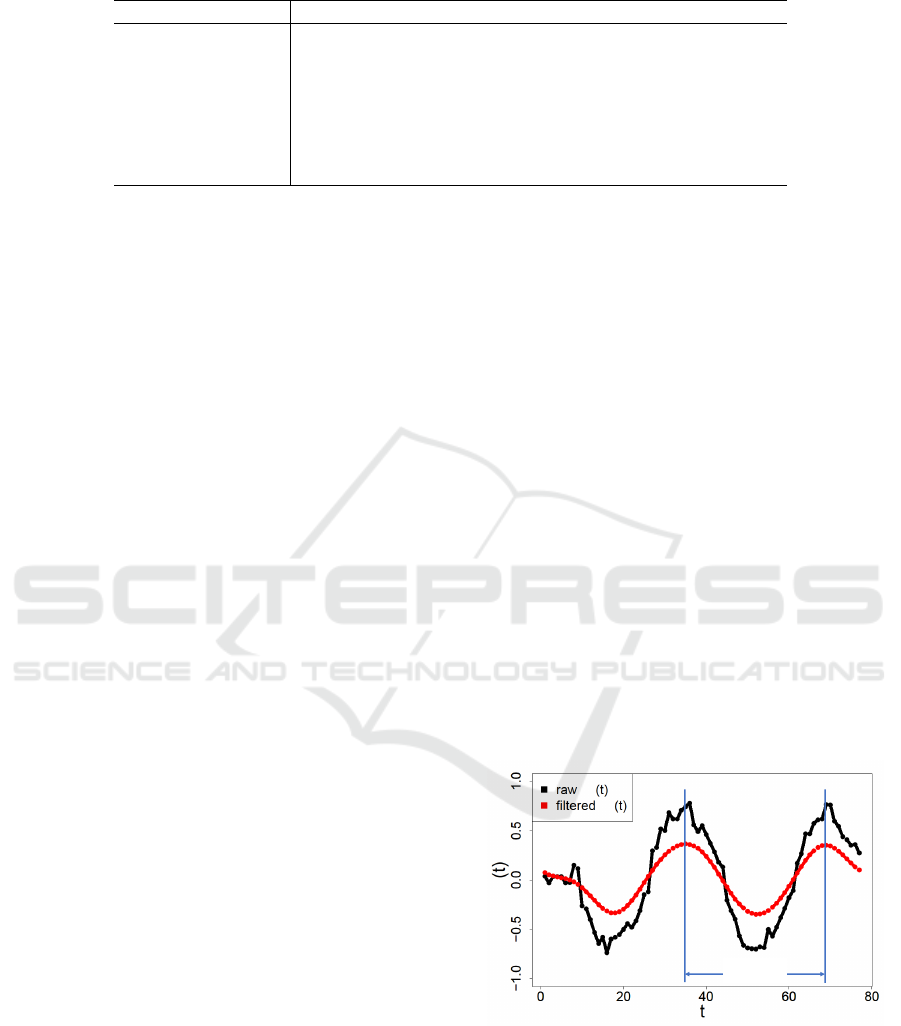
Table 1: Differences between the present work and previous works.
Muaaz GEI Mori 2018 This work
No. of features 1 1 1-36 1-24
Sensor inner outer outer outer
Observation period long short short short
No. of templates multi N/A single single
Target cooperation necessary unnecessary unnecessary unnecessary
Method DTW dist. GEI statistic feature DTW dist.
No. of subjects
35 - 10 31
rank-1 accuracy is 95.8% and the EER is 0.022.
2.1 Dynamic Time Warping
The DTW algorithm is a well-known method for pat-
tern matching and is used in speech recognition. It
quantifies the distance differences between two sets
of time series data with different lengths. A DTW
distance between two sets of time series data P =
(p
1
, p
2
,..., p
n
P
) and Q = (q
1
,q
2
,...,q
n
Q
), denoted by
d(P,Q), is defined as
d(P,Q) = f (n
P
,n
Q
), (1)
where, f (i, j) is calculated recursively as
f (i, j) = ||p
i
− q
j
|| + min
f (i, j − 1), f (i − 1, j),
f (i − 1, j − 1),
(2)
f (0,0) = 0, f (i,0) = f (0, j) = ∞. (3)
The DTW algorithm also has many other uses.
Lee et al. proposed a handwritten pattern recogni-
tion method using the DTW algorithm on motion sen-
sor data generated from an accelerometer and a gy-
roscope (Lee et al., 2018). In this work, the accuracy
of the proposed method was 91.4% using a real-world
data set.
Li et al. proposed a gait recognition method based
on human electrostatic signals (Li et al., 2018). The
authors used DTW on the electric signal of walking.
From their experiment, the best correct rate achieved
was 87.5%.
3 PROPOSED METHOD
In this work, we recognize a person by using 3-
dimensional coordinates observed by motion capture
sensors, and calculate the DTW distance of the time
series data of one cycle of walking. The proposed
method consists of four steps:
1. Cycle extraction
2. Calculation of relative coordinates
3. Calculation of DTW distance
4. Person recognition.
3.1 Cycle Extraction
Let a
`
(t) = (x,y,z) be a time series of 3-dimensional
absolute coordinates of joint ` in time t. Skeleton data
is a set of time series data of absolute coordinates in
time t.
We extract one cycle of walking from the skeleton
data. In our environment, an observed video stream
contains about two cycles.
First, let ∆(t) be the distance between both feet in
time t, defined using a
LF
(t) and a
RF
(t) as
∆(t) = ±||a
RF
(t) − a
LF
(t)||. (4)
If the right foot is in front, the sign of ∆(t) is positive,
otherwise it is negative.
Next, the Fourier transformation is applied to the
time series ∆(1),...,∆(n) and a low pass filter is ap-
plied to reduce noise and detect one cycle. The re-
sulting 1/30 low-frequency components are proces-
sed later. We define a cycle of walking as the period
between peaks. Note that the low pass filter is used
only for the purpose of cycle extraction and we use
non-filtered data for the DTW algorithm. The origi-
nal data and filter-applied data are shown in Figure 1.
1 cycle
Δ
Δ
Δ
Figure 1: Distance between foot (black) and that of applied
low pass filter (red).
In the cycle extraction phase, time t is a unit cor-
responding to the frame rate of the motion capture
sensor. For example, Figure 1 shows example data
for 2.6 seconds where the frame rate is 30 fps. We
see noise-containing data (black) translated into gra-
dually changing data (red). In these example data, we
Robust Person Identification based on DTW Distance of Multiple-Joint Gait Pattern
223

have one cycle as a series of features from the first
peak (t = 37) to the second peak (t = 70). The data is
normalized from t
1
to t
35
.
3.2 Calculation of Relative Coordinates
We calculate relative coordinates of joints while wal-
king. The origin of coordinates is chosen from stable
joints in the center of the body. Note that in the expe-
riment in Section 4, c is SpineMid.
Let a
c
(t) be an absolute coordinate of center joints
c at time t. The relative coordinate r is defined as
r
`
(t) = a
`
(t) − a
c
(t). (5)
3.3 Calculation of DTW Distance
We use a DTW algorithm to calculate a distance of
time series data. In our study, the position of a joint
is defined in three axes, so we use multi-dimensional
dynamic time warping (MD-DTW) (ten Holt et al.,
2007). In MD-DTW, the 3-dimensional Euclidian dis-
tance is defined as
||p
i
− q
j
|| =
q
(p
i,x
− q
j,x
)
2
+ (p
i,y
− q
j,y
)
2
+ (p
i,z
− q
j,z
)
2
.
(6)
Let R
`
= hr
`
(t
1
),...,r
`
(t
n
)i and R
0
`
=
hr
0
`
(t
1
),...,r
0
`
(t
n
0
)i be the time series data of joint `.
Let d(R,R
0
) be the distance between R and R
0
. When
R = R
0
, d(R, R
0
) = 0. It is not necessary to assume
that n = n
0
, but n is distributed in almost the same
way because the data is normalized in Section 3.1.
When several features are aggregated, the distance
is calculated as follows. Given two data sets (R
`
,R
m
)
and (R
0
`
,R
0
m
), and data of joints ` and m, an integra-
ted DTW distance D
(R
`
,R
m
),(R
0
`
,R
0
m
)
is defined
as an Euclidian distance of all DTW distances. i.e.,
p
d(R
`
,R
0
`
)
2
+ d(R
m
,R
0
m
)
2
. Likewise, given k featu-
res, distances are calculated as a k-dimensional Euc-
lidian distance.
3.4 Person Recognition
Let U be the set of all users. Let R
(u)
be time series
data of k pieces of normalized relative coordinates of
user u. Given s pieces of data (R
u
1
,...,R
u
s
), let tem-
plate data R
(u)
∗
be one of them. It is regarded that
u = v, if the integrated DTW distance D(R
(u)
,R
(v)
)
of the two sets of time series data R
(u)
and R
(v)
is less
than θ.
Threshold θ
∗
`
is determined using the EER. Let
W
(u)
= {R
(u)
1
,...,R
(u)
s
} be a set of time series data
of u. At this time, the FRR and FAR are calculated as
FRR(θ,u) =
|{R
(u)
∈ W
(u)
|D(R
(u)
,R
(u)
∗
) > θ}|
|W
(u)
|
, (7)
FRR(θ) =
1
|U|
∑
u∈U
FRR(θ,u), (8)
FAR(θ,u) =
|{R ∈ W −W
(u)
|D(R,R
(u)
∗
) ≤ θ}|
|W
(u)
|
. (9)
FAR(θ) =
1
|U|
∑
u∈U
FAR(θ,u), (10)
At this point, W is a set of time series data of all users.
The EER is an average error rate using threshold θ
∗
`
such that FAR(θ
∗
`
) = FRR(θ
∗
`
).
4 EXPERIMENT
4.1 Experiment Purposes
The purposes of our experiment are as follows:
1. To identify the best parameters (choice of num-
ber of joints k and threshold θ
∗
) for the proposed
gait identification method using skeleton data and
DTW.
2. To evaluate the basic accuracy of the proposed
method.
3. To evaluate the accuracy of the proposed method
for walking containing some obstacles.
4. To identify the obstacle-robust joints.
4.2 Motion Capture Device
We used the Kinect V2, a motion capture device de-
veloped by Microsoft.
The Kinect device includes an RGB camera,
a depth camera, and a microphone. It identifies
three-dimensional coordinates of joints of the player
to recognize the player’s movements. The three-
dimensional coordinates captured by the Kinect de-
vice are called skeleton data and can be retrieved via
the Kinect Software Development Kit.
4.3 Experimental Method
4.3.1 Experiment 1: Normal Walking
We captured walking data using Kinect V2 and eva-
luated the accuracy of the proposed method. We used
31 subjects, and each subject was assigned an ID from
ICISSP 2019 - 5th International Conference on Information Systems Security and Privacy
224
Table 2: Information on the experiment.
1: Normal 2: Obstacles
Date April 19, 2018 March 26, 2018
Start time 12:40 19:00
End time 14:50 21:15
#subjects 31 5
Sex 26 male, 5 female 5 male
#walks 5 2
Age
18–51 21–24
Place classroom laboratory
1–31. Information regarding this experiment, Experi-
ment 1, is shown in Table 2.
We observed some skeleton data
a
1
(t),...,a
25
(t)
for walking straight in the
environment, as shown in Figure 2. The Kinect
device was placed horizontally 0.9 m above the floor.
The subjects each walked five times from a distance
of 5.5 m away to 1 m away from the device.
0.9m
0m
5.5m
4.5m
2m1m
Start
Walking
Start
Recording
Finish
Recording
Finish
Walking
Kinect
Figure 2: Environment of Experiment 1.
In this experiment, we used SpineMid as the
origin c. Relative coordinates of joints from c
were calculated. We calculated the DTW distance
d
R
(u)
`
,R
(v)
`
for each ` and detected the optimal θ
∗
`
for minimizing the EER.
We calculated the integrated DTW distance of the
top k joints in descending order of the EER and eva-
luated the EER.
4.3.2 Experiment 2: Obstacle-Containing
Walking
Some samples of obstacles are illustrated in Figure 3.
The information for data capture for this experiment,
Experiment 2, are shown in Table 2. We applied the
following 12 obstacles:
1. Normal (no obstacle),
2. Swinging hand and foot in a big swing (b-swing),
3. Swinging hand and foot in a small swing (s-
swing),
4. Putting hands in front pocket (pocket),
5. Walking while looking at smartphone (phone),
6. Carrying a handbag (handbag),
7. Carrying a shoulder bag (shoulder bag),
Figure 3: Sample obstacles (2 (b-swing), 4 (pocket), 5
(phone), 8 (sack), 9 (umbrella), 10 (box), 11 (sandals), 12
(suitcase)).
8. Carrying a knapsack (sack),
9. Holding an umbrella (umbrella),
10. Carrying a large box (box),
11. Wearing sandals (sandals),
12. Pulling a suitcase (suitcase).
We selected one set of template data from normal
walking and calculated the integrated DTW distance
with obstacle-containing data.
4.4 Experimental Results
4.4.1 Data Capture
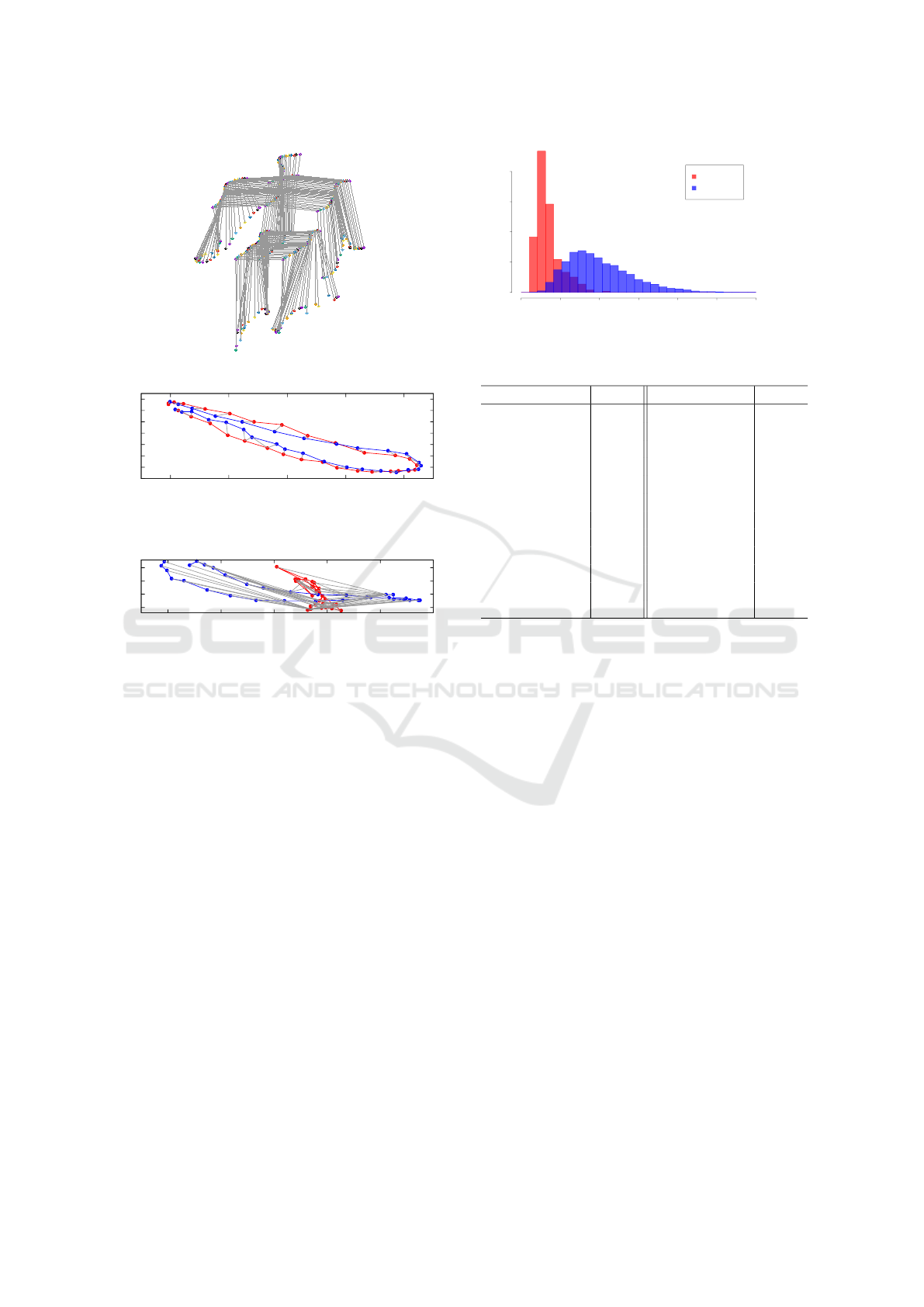
A sample of a 3D plot is shown in Figure 4. We show
the one-cycle trace of 11 principal joints (Head, Spi-
neShoulder, ShoulderRight, ShoulderLeft, HandTi-
pRight, HandTipLeft, SpineBase, HipRight, HipLeft,
FootRight, FootLeft). The subject was a 24-year old
male. He walked horizontally, swinging his head. In
this sample, one cycle had 33 frames and lasted 1.1
seconds.
4.4.2 DTW Distance
As an example, we show the sample calculation pro-
cesses of the DTW distance for HandTipLeft in Fi-
gure 5 and 6. The red line shows the trace on the x
and y axes of the movement of HandTipLeft of walk
1, and the blue line is that of walk 2. Matched coor-
dinates are indicated with gray lines. Figure 5 shows
Robust Person Identification based on DTW Distance of Multiple-Joint Gait Pattern
225
2 Kinect v2
RGB 1920×1080
RGB 30fps
512×424
30fps
6
6
25
0.54.5m
2 Kinect v2 [9]
3
2018/4/19
31
5
0.9m
0m 5.5m
4.5m
2m1m
Kinect
3 1
3
3
Kinect 0.9m
Kinect 5.5m 1m
4.5m 2m
4.3.2
24 DTW
0.8
1
1.2
1.4
1.6
1.8
2
2.2
2.4
2.6
2.8
3
-1
-0.5
0
0.5
1
-1
-0.5
0
0.5
1
4 1 3D
Distance
Density
0 2 4 6 8 10 12
0.0 0.2 0.4 0.6 0.8 1.0
Self
Others
5 HAND TIP LEFT DTW
FAR FRR EER
24 EER
EER
4.4
4.4.1
1 4
4.4.2
31 5 DTW
HandTipLeft 5
Head, HandTipLeftHandTipRightFootLeft
FootRight 5
6
24 EER
4
4 n EER
7 n =5 EER
0.036 n =6
EER 5
ROC 8
c
⃝ 2018 Information Processing Society of Japan
Figure 4: Change of skeleton data a(t) of one cycle.
-0.32
-0.3
-0.28
-0.26
-0.24
-0.22
-0.2
-0.18
-0.3 -0.2 -0.1 0 0.1
Figure 5: DTW distance of HandTipLeft (genuine)
d(R
(u)
HT L
,R
0(u)
HT L
)
.
-0.3
-0.25
-0.2
-0.15
-0.6 -0.4 -0.2 0 0.2 0.4
Figure 6: DTW distance of HandTipLeft (impostor)
d(R
(u)
HT L
,R
0(v)
HT L
)
.
the result of the DTW process for a genuine person
and Figure 6 shows the results of an impostor.
For the genuine person, the DTW distance, defi-
ned as the sum of the gray lines, d
R
(u)
HT L
,R
0(u)
HT L
=
0.45. Thus, it implies that the trace of the left hand
differed 1.5 cm in 1/30 second because one cycle has
30 frames, as shown in Figure 5.
In contrast, for the impostor data, there is a signi-
ficant difference between user u and v. In Figure 5,
d
R
(u)
HT L
,R
(u)
HT L
= 12.0.
As examples, the distribution of DTW distances
of HandTipLeft (HTL) d
R
(u)
HT L
,R
(v)
HT L
is shown in
Figure 7. In both graphs, the genuine (red) data are
distributed closer than the impostor (blue) data and
are distributed in a smaller range. The overlapped
area is equal to the sum of the FAR and the FRR.
A DTW distance is determined when both error ra-
tes are equal. According to this result, θ
∗
HT L
= 2.19.
Other joints were distributed similarly to the HTL and
SL joints. The sorted EERs of all joints are shown in
Table 3.
From Figure 3, we find:
1. The EERs of the Neck, Head and Shoulder-
DTW Distance d(R,R)
Density
0 2 4 6 8 10 12
0.0 0.2 0.4 0.6 0.8
genuine
impostor
Figure 7: Distribution of DTW distance of HTL.
Table 3: EER of 24 Joints.
Joint EER Joint EER
ElbowLeft 0.076 HandRight 0.124
ShoulderRight 0.081 HipLeft 0.127
ShoulderLeft 0.095 WristRight 0.133
Neck 0.100 HandTipRight 0.133
SpineShoulder 0.100 FootRight 0.144
WristLeft 0.107 KneeRight 0.145
HipRight 0.107 AnkleRight 0.148
HandLeft 0.108 KneeLeft 0.155
Head 0.110 ThumbRight 0.177
HandTipLeft 0.112 ThumbLeft 0.187
ElbowRight 0.113 AnkleLeft 0.187
SpineBase 0.123 FootLeft 0.192
Right/Left tended to be stable.
2. With regard to the joints in the arms (Elbow,
Wrist, Hand), the joints in the left arm were more
stable than those in the right arm.
3. The EERs of joints in the legs (Foot, Knee, Ankle)
tended to be unstable.
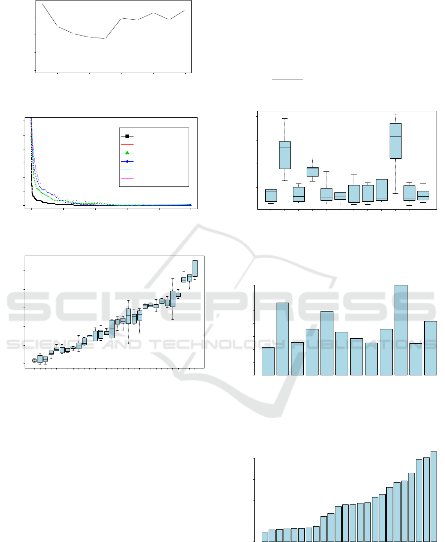
4.4.3 Calculation of Integrated DTW Distance
We aggregated the top k joints (1 ≤ k ≤ 10) in Ta-
ble 3 to improve accuracy. We show the change of the
integrated EERs in Figure 8. We find that the EER de-
creases as the number of aggregated joints increases.
When k is five or less, the minimum EER is 0.036.
When k is six or more, the EER does not decrease.
Therefore, k = 5 is regarded as the optimum value.
Hereafter, we used the following five joints: Elbo-
wLeft (EL), ShoulderRight (SR), ShoulderLeft (SL),
Neck (NK), and SpineShoulder (SS).
We show the receiver operating characteristic
(ROC) curves of the top five joints in Figure 9. The
black line shows the ROC of the combined five joints
and the others show the five individual joints. The
diagonal line in the figure shows the EER. From this
figure, the integrated DTW distance has a lower EER
than the single joints.
We calculated the integrated DTW distance of the
ICISSP 2019 - 5th International Conference on Information Systems Security and Privacy
226
●
●
●
●
●
●
●
●
●
●
2 4 6 8 10
0.00 0.02 0.04 0.06
k
EER
Figure 8: EER of integrated DTW distance.
0.0 0.2 0.4 0.6 0.8 1.0
0.0 0.2 0.4 0.6
FRR
FAR
●
●
●
●
●
●
●
●
●
●
●
●
●
●
●
●
●
●
●
●
●
●
●
●
●
●
●
●
●
●
●
●
●
●
●
●
●
●
●
●
●
●●
●
●
●●
●●
●●
●
●●●
●
●
●●●●
●●●
●●
●●
●
●
●●●
●●●
●●●
●●
●●●●●●●●●●●●●●●●●●●●
●●●●●
●●●●●
●●●●●●●●●●●●●●●
●●●●●●●●●●●●●●●●●●●●●●●●●●●●
●●●●●●●●●●●●●●●●●●●●●●●●●●●●●●●●●●●●●●●●●●●●●●●●●●●●●●●●●●●●●●●●●●●●●●●●●●●●●●●●●●●●●●●●●●●●●●●●●●●●●●●●●●●●●●●●●●●●●●●●●●●●●●●●●●●●●●●●●●●●●●●●●●●●●●●●●●●●●●●●●●●●●●●●●●●●●●●●●●●●●●●●●●●●●●●●●●●●●●●●●●●●●●●●●●●●●●●●●●●●●●●●●●●●●●●●●●●●●●●●●●●●●●●●●●●●●●●●●●●●●●●●●●●●●●●●●●●●●●●●●●●
0.0 0.2 0.4 0.6 0.8 1.0
0.0 0.2 0.4 0.6
FRR
FAR
0.0 0.2 0.4 0.6 0.8 1.0
0.0 0.2 0.4 0.6
FRR
FAR
0.0 0.2 0.4 0.6 0.8 1.0
0.0 0.2 0.4 0.6
FRR
FAR
●
●
●
●
●
●
●
●
●
●
●
●
●
●
●
●
●
●
●
● ●
● ●
●
●
●
●
●
●
●
●
● ● ● ● ●
●
●
● ● ●
● ● ● ● ●
● ● ● ● ● ● ● ● ●
●
● ● ● ● ● ● ●
● ● ● ● ● ● ● ●
●
●● ●●●●●●●●●●●●●●●●●●●●●●●●●●●●●●●●●●●●●●●●●●●●●●●●●●●●●●●●●●●●●●●●●●●●●●●●●●●●●●●●●●●●●●●●●●●●●●●●●●●●●●●●●●●●●●●●●
0.0 0.2 0.4 0.6 0.8 1.0
0.0 0.2 0.4 0.6
FRR
FAR
●
●
●
●
●
●
●
●
●
●
●
●
●
●
●
●
● ●
●
●
●
●
●
●
●
●
● ● ●
● ●
●
● ● ●
● ● ● ● ● ● ● ●
●
● ● ● ●
● ● ● ● ● ●
● ●
● ● ● ● ● ● ● ● ● ● ● ● ● ● ● ● ● ● ●●● ● ●●●●●●●●●●●●●●●●●●●●●●●●●●●●●●●●●●●●●●●●●●●●●●●●●●●●●●●●●●●●●●●●
0.0 0.2 0.4 0.6 0.8 1.0
0.0 0.2 0.4 0.6
FRR
FAR
●
●
●
Euclid
ElbowLeft
ShoulderRight
ShoulderLeft
Neck
SpineShoulder
Figure 9: ROC curves.
●
●
●
●
●
●
●
●
●
●
●
●
U13
U23
U21
U20
U10
U17
U6
U4
U26
U2
U24
U18
U16
U5
U1
U8
U7
U9
U30
U22
U29
U27
U3
U25
U12
U19
U14
U11
U15
U28
1.5 2.0 2.5 3.0 3.5 4.0
DTW Dist.
Figure 10: Distribution of the integrated DTW distance of
all subjects.
top five joints between U31. We show the boxplot of
the result in Figure 10. U31 is regarded as the average
user. The range and quartiles of the integrated DTW
distance for the 30 users are sorted by the mean va-
lues. Some users have similar distances, but we can
distinguish them.
4.4.4 Obstacle Walking
We calculated the DTW distance of obstacle-
containing walking
d(R
(u)
normal
,R
(u)
)
. The means of
the DTW distances are shown in Table 4, where the
largest value in each obstacle is underlined. We found
that all obstacles increased the EER above the nor-
mal EERs. The obstacle with the most underlined
DTW distances is the box. The B-swing affects the
Foot (FootR/L) substantially, and the suitcase affects
the Shoulder (SR/SL). The box increases the EER
from 3.46 to 14.278, which is 4.1 times greater. On
average, the box increases the EER to 1.13 (2.95 ti-
mes greater).
The distributions of the DTW distances for HTL
d
R
(u)
HT L
,R
0(u)
HT L
for each obstacle is shown in Figures
11, respectively. In addition, the averages of the DTW
distances d(R,R
0
) for each obstacle and each joint are
shown in Figures 12 and 13, respectively.
●
●
●
●
normal
b−swing
s−swing
pocket
phone
handbag
shoulder bag
sack
umbrella
box
sandals
suitcase
5 10 15 20
DTW Dist.
Figure 11: Distribution of DTW distances for HTL
d
R
(u)
HT L
,R
0(u)
HT L
for each obstacle.
normal
b−swing
s−swing
pocket
phone
handbag
shoulder bag
sack
umbrella
box
sandals
suitcase
Distance
0 1 2 3 4 5 6 7
Figure 12: Mean of DTW distances d
R
(u)
,R
0(u)
for each
obstacle.
SpineShoulder
Neck
SpineBase
ShoulderRight
ShoulderLeft
HipLeft
HipRight
Head
KneeLeft
ElbowLeft
AnkleLeft
ElbowRight
AnkleRight
KneeRight
FootLeft
FootRight
WristLeft
HandLeft
ThumbLeft
HandTipLeft
WristRight
HandRight
ThumbRight
HandTipRight
Distance
0 2 4 6 8
Figure 13: Mean of DTW distance d
R
(u)
,R
0(u)
for each
joint.
Robust Person Identification based on DTW Distance of Multiple-Joint Gait Pattern
227
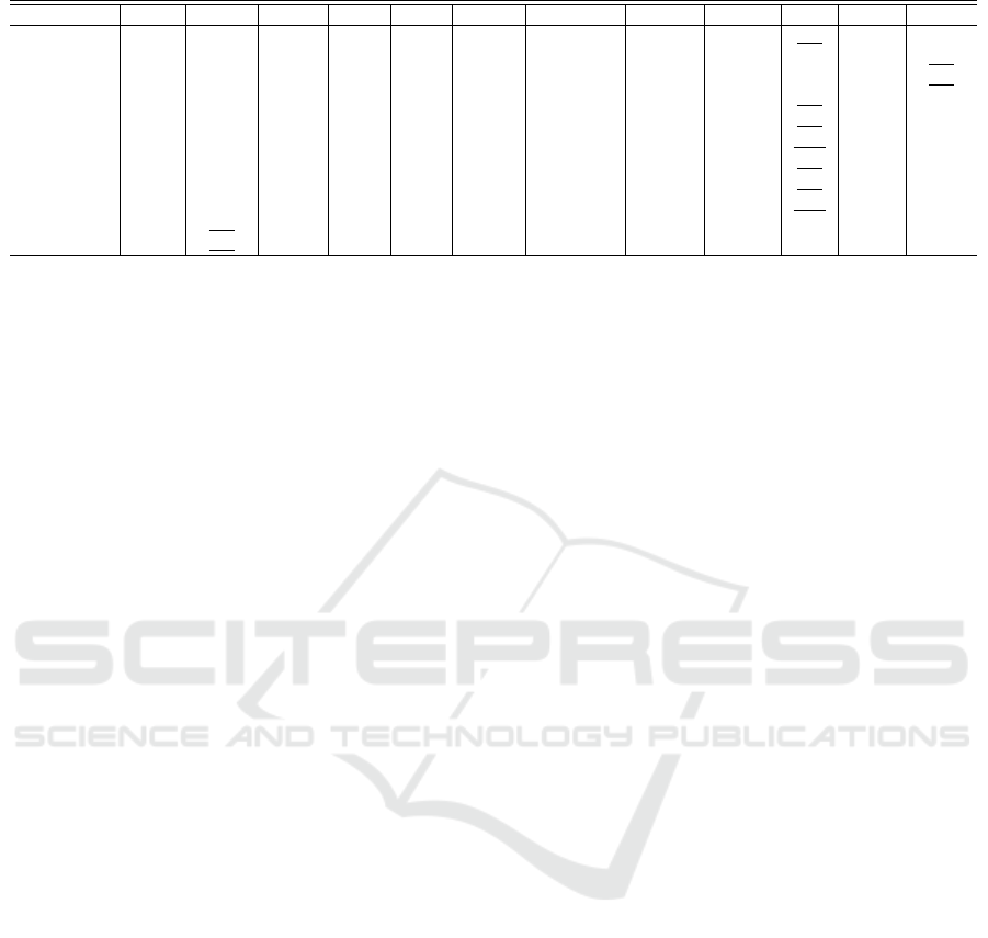
Table 4: Means of DTW distance d(R,R
0
) of each joint for each obstacle.
normal b-swing s-swing pocket phone handbag shoulder bag knapsack umbrella box sandals suitcase
ElbowLeft 1.83 5.41 1.83 3.06 2.36 2.18 1.86 1.88 2.48 5.61 1.68 2.28
ShoulderRight 0.97 1.76 0.99 0.96 1.06 1.31 1.33 1.14 1.12 1.60 0.99 1.63
ShoulderLeft 0.98 1.38 1.00 1.23 1.43 1.44 1.31 1.24 1.03 1.59 1.01 1.71
HipRight 0.95 1.44 1.13 1.11 1.13 1.56 1.62 1.04 1.18 1.89 1.13 1.67
Head 0.92 1.60 1.18 1.20 1.82 1.56 1.74 1.09 1.37 2.57 1.09 1.43
HandTipLeft 3.46 12.85 3.60 8.59 3.90 3.79 3.40 3.29 5.98 14.27 3.44 3.47
ElbowRight 1.84 4.55 2.28 2.92 4.20 3.17 2.76 2.47 3.52 6.90 2.15 5.83
HipLeft 1.09 1.39 1.16 1.14 1.14 1.23 1.50 1.16 1.27 2.21 1.10 1.39
HandTipRight 3.18 9.28 3.84 6.48 20.85 7.76 5.61 4.02 8.19 18.06 3.94 12.50
FootRight 3.31 6.91 4.39 3.48 3.68 3.95 4.12 4.41 4.03 4.46 4.13 4.55
FootLeft
2.96 6.32 3.89 3.15 2.88 3.27 3.21 3.70 3.69 4.14 4.06 3.80
From Figure 12, obstacles decrease the accuracy.
The most influential obstacle is carrying a box. From
Figure 13, obstacle-robust joints are the Shoulder,
Head, and Hip. In particular, the most robust joint
is the SpineShoulder.
5 DISCUSSION
In Experiment 1, stable joints have lower EERs than
variable joints. This is because the distribution of sta-
ble joints in a particular person falls in a very small
interval. Even when it is close to that of other persons,
it can be an effective feature to recognize persons. We
claim that stable joints, e.g., the head and the shoul-
ders, move periodically in a very small range.
From Table 3, in the upper half of the body, joints
on the left side have a lower EER than those on the
right side. We think the reason for this is that some
users swing their arms somewhat like the red line in
Figure 6. Joints that swing a little are more stable and
stable joints tend to be useful features.
In Figure 8, we suggest that the EER decreases as
the number of aggregated joints increases. When k is
five or less it is estimated that the dimension of the
feature is increasing and the difference between dif-
ferent persons becomes greater. However, when inte-
grated over six joints, we think the features have too
many dimensions and repeatability in the same user
decreases, which results in the EER increasing.
Big swings and carrying boxes are the largest ob-
stacles. In particular, joints in the arms are affected
by these obstacles significantly. However, we consi-
der that big swings of arms and carrying big boxes do
not occur often in daily life. Therefore, we claim that
the proposed method is robust in terms of obstacles.
6 CONCLUSIONS
In this work, we proposed a new person identification
method using time series data of 3-dimensional joint
coordinates, captured by a depth sensor. As a result
of our experiments, we decreased the EER to 0.03 by
using five joints including ElbowLeft, ShoulderRight,
ShoulderLeft, Neck and SpineShoulder. This is con-
siderably lower than that obtained by previous works,
such as (Mori and Kikuchi, 2018) (0.25) or (Muaaz
and Mayrhofer, 2017) (0.13).
We verified the accuracy of the proposed system
using obstacle-containing walking data. As a result,
stable joints such as the shoulder or head are not af-
fected by obstacles.
REFERENCES
Berndt, D. J. and Clifford, J. (1994). Using dynamic time
warping to find patterns in time series. The Third In-
ternational Conference on Knowledge Discovery and
Data Mining, pages 359–370.
Han, J. and Bhanu, B. (2006). Individual recognition using
gait energy image. IEEE Trans. Pattern Anal. Mach.
Intell., 28(2):316–322.
Igual, L., Lapedriza, A., and Borr
`
as, R. (2013). Robust
gait-based gender classification using depth cameras.
EURASIP Journal on Image and Video Processing,
2013(1):1–11.
Lee, W.-H., Ortiz, J., Ko, B., and Lee, R. (2018). Inferring
smartphone usersf handwritten patterns by using mo-
tion sensors. 4th International Conference on Infor-
mation Systems Security and Privacy, pages 139–148.
Li, M., Chen, X., Tian, S., Wang, Y., and Li, P. (2018).
Research of gait recognition based on human electro-
static signal. 2018 2nd IEEE Advanced Information
Management,Communicates,Electronic and Automa-
tion Control Conference (IMCEC), pages 1812–1817.
Mori, T. and Kikuchi, H. (2018). Person tracking based on
gait features from depth sensors. The 21st Internati-
onal Conference on Network-Based Information Sys-
tems (NBiS-2018), 22:743–751.
ICISSP 2019 - 5th International Conference on Information Systems Security and Privacy
228

Muaaz, M. and Mayrhofer, R. (2017). Smartphone-
based gait recognition: From authentication to imi-
tation. IEEE Transactions on Mobile Computing,
16(11):3209–3221.
Preis, J., Kessel, M., Werner, M., and Linnhoff-Popien, C.
(2012). Gait recognition with kinect. Proceedings of
the First Workshop on Kinect in Pervasive Computing.
Shiraga, K., Makihara, Y., Muramatsu, D., Echigo, T., and
Yagi, Y. (2016). Geinet: View-invariant gait recogni-
tion using a convolutional neural network. 2016 Inter-
national Conference on Biometrics (ICB), pages 1–8.
Sklavos, N. and Souras, P. (2006). Economic models and
approaches in information security for computer net-
works. International Journal of Netowk Security,
2(1):14–20.
ten Holt, G. A., Reinders, M. J. T., and Hendriks, E. A.
(2007). Multi-dimensional dynamic time warping for
gesture recognition. Thirteenth annual conference of
the Advanced School for Computing and Imaging.
Zhang, Y., Pan, G., Jia, K., Lu, M., Wang, Y., and Wu,
Z. (2015). Accelerometer-based gait recognition by
sparse representation of signature points with clusters.
IEEE Transactions on Cybernetics, 45:1864–1875.
Robust Person Identification based on DTW Distance of Multiple-Joint Gait Pattern
229
