Visibility Forecast for Airport Operations by LSTM Neural Network

Tuo Deng

, Aijie Cheng

, Wei Han

and Hai-Xiang Lin

School of Mathematics, Shandong University, Jinan, Shandong, 250100, China

Numerical Weather Prediction Center of China Meteorological Administration, Beijing, 100081, China

Delft Institute of Applied Mathematics, Delft University of Technology, Mekelweg 4, 2628 CD Delft, Netherlands

Keywords:

Atmospheric Visibility, Time Series Forecast.

Abstract:

Visibility forecast is a meteorological problems which has direct impact to daily lives. For instance, timely

prediction of low visibility situations is very important for the safe operation in airports and highways. In this

paper, we investigate the use of Long Short-Term Memory(LSTM) model to predict visibility. By adjusting

the loss function and network structure, we optimize the original LSTM model to make it more suitable for

practical applications, which is superior to previous models in short-term low visibility prediction. In addition,

there is a ”time delay problem” when the number of hours time ahead we try to forecast becomes larger, this

problem is persistent given the limited amount of available training data. We report our attempt of applying

re-sampling to deal with the time delay problem, and we ﬁnd that this method can improve the accuracy of

visibility prediction, especially for the low visibility case.

1 INTRODUCTION

Atmospheric visibility is the maximum horizontal

distance that a person with normal vision can distin-

guish the target with sky as the background, which

is an important indicator to reﬂect the degree of air

pollution (Fan et al., 2016). In the case of rain and

snow and severe smog, the visibility can be very low,

which will greatly affect the safety of aviation, na-

vigation and highway trafﬁc. Visibility is inﬂuenced

by a variety of meteorological factors, such as tempe-

rature, wind, precipitation, pressure, etc. In particu-

lar, visibility shows strongly correlation with relative

humidity, PM2.5, PM10 and so on. Traditional pre-

diction methods relying on physical modeling are in-

effective due to the complexity and inability to fully

quantify the inﬂuence of many different factors. For

instance, Clark et al. have investigated the problem of

prediecting visibility by numerical methods with the

Operational Met Ofﬁce Uniﬁed Model(Clark et al.,

2008). The results are not very accurate, especially

in case of low visibility due to insufﬁcient spatial re-

solution of the numerical grid. Visibility can change

abruptly in a scale of 10m, whereas the current nume-

rical NWP models have a spatial resolution of 10km.

Currently, there are two main approaches to pre-

dict the visibility. The ﬁrst approach is based on

the numerical forecast of other meteorological fac-

tors, and then calculates the visibility based on some

empirical relationship with those factors. Most pre-

vious researches are following such approach, and

the methods of empirical ﬁtting the interrelation bet-

ween elements are mainly based on polynomial ﬁtting

and traditional machine learning model. The polyno-

mial relationship between visibility, relative humidity

and aerosol concentration has been studied in the ci-

ties such as Shijiazhuang (Wang et al., 2016), Tianjin

(Song et al., 2013) and Hangzhou (Fan et al., 2016).

The visibility for highway in foggy weather is ﬁt-

ted by temperature, wind speed and humidity through

SVM and BP neural network (Long et al., 2017) in

past studies. However, the prediction results of these

methods are not accurate, and can only predict the ge-

neral trend of visibility changes.

The second approach is to treat the visibility over

a period of time as a time series (Dietterich, 2002),

and solve the problem of time series prediction with

methods of machine learning or deep learning. For

instance, regression tree (Dietz et al., 2017) and MLP

(Zhu et al., 2017) are studied for airport visibility fo-

recast.

These two kinds of methods have their own ad-

vantages and disadvantages. The ﬁrst method has bet-

ter interpretability due to the application of the actual

physical model, but it is inaccurate due to the com-

plexity and the lack of full understanding of the phe-

466

Deng, T., Cheng, A., Han, W. and Lin, H.

Visibility Forecast for Airport Operations by LSTM Neural Network.

DOI: 10.5220/0007308204660473

In Proceedings of the 11th International Conference on Agents and Artiﬁcial Intelligence (ICAART 2019), pages 466-473

ISBN: 978-989-758-350-6

nomenon. Besides, this method is highly dependent

on the prediction accuracy of other meteorological

elements. The second method only uses the meteo-

rological data as input and few physical information

as prior knowledge, which makes the model much

simpler. However, it does not deliver an explanation

about the relationship between meteorological factors

and the actual physical laws.

In the past two decades, machine learning has at-

tracted much attention and established their position

as important competitors of classical statistical in the

ﬁeld of prediction (Kurt and Oktay, 2010). A num-

ber of methods have been widely used, such as SVM,

KNN, Decision Trees, etc (Friedman et al., 2001).

These methods use only historical data to learn the

random dependencies between the past and the fu-

ture. Among these methods, Recurrent Neural Net-

work(RNN) can capture the characteristic of data in

sequence problems. Particularly, it has been applied

in time-series forecast problem (Yadav et al., 2013).

However, RNN models have their own shortco-

mings. Traditional RNN models can not capture long-

term dependencies in the sequence of input data. To

solve this problem, Long short-term memory(LSTM)

neural network was developed. Compared with tra-

ditional RNN models, LSTM can avoid the problem

of gradient vanishing and caputre the long-term de-

pendencies in time-series forecast problems. It has

been used in many ﬁelds, such as air pollutant pre-

diction (Li et al., 2017), earthquake prediction (Wang

et al., 2017), stock price prediction (Minami, 2018)

and internet trafﬁc prediction (Cortez et al., 2006),

etc. LSTM has also been used for visibility prediction

in previous studies(Salman et al., 2018). However, the

result is of limited practical signiﬁcance since they

focused only on overall errors(RMSE) and did not

pay attention to the accuracy of low-visibility fore-

cast, which is precisely the most relevant and difﬁcult

part in practical application.

This paper aims to use LSTM to make visibility

predictions which is a problem with properties dif-

ferent from the aforementioned applications. Speci-

ﬁcally, we consider visibility forecast of 1 hour re-

spectively and 3 hours ahead. Compared with the

commonly used visibility prediction models in previ-

ous studies, the LSTM model has signiﬁcantly impro-

ved, which is more accurate in cases of low visibility.

Because low visibility is more concerned in practice,

we design a weighted loss function to optimize the

model. In order to make predictions of many hours

more(e,g., 6 or 8 hours ahead), we ﬁnd that there is

a systematic time delay in forecast result, which can

be caused by insufﬁcient data. This also leads to the

inability of visibility prediction models to make accu-

rate predictions for 24-hour or longer like some areas

mentioned above. We try to ﬁx it by resampling.

2 DATA AND ANALYSIS

In this section, we describe the speciﬁc information

of data, which contains the elements and distribution

of data. The spatiotemporal correlation of data is also

analyzed. Besides, we ﬁx the missing values through

spatial correlation and normalize the data. In addi-

tion, for the particularity of time series, we need to

reconstruct the input data.

2.1 Data Description

The data that we used is provided by China Meteo-

rological Administration(CMA). Speciﬁcally, we use

the meteorological data of Beijing station ’54511’

from April 2016 to December 2017, which contains

15143 sets of data. Each set corresponds to hourly

measurements, including PM10, PM2.5, temperature,

precipitation, pressure, relative humidity, wind speed,

wind direction and visibility. We choose the ﬁrst

10000 sets of data as training set while the remaining

data as test set to verify the model. Spatially, we se-

lect ten sites with relatively complete data around Bei-

jing, among which Beijing station 54511 is chosen as

experimental data to construct time series, and the re-

maining nine sites are used to interpolation missing

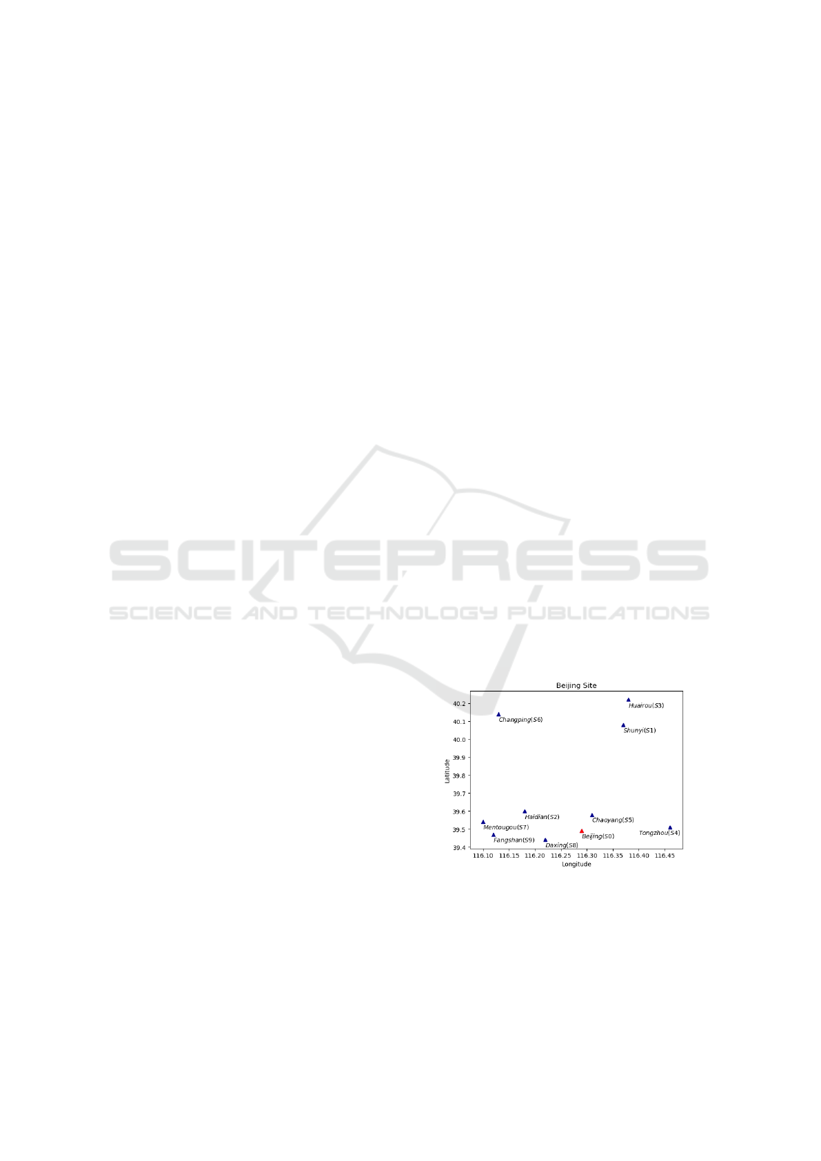
data. Figure 1 shows the location of all ten meteoro-

logical observation stations that we use, and Beijing

station is marked in red.

Figure 1: Location of stations in Beijing.

In order to understand the distribution of data bet-

ter, we segment the existing data into bar charts in

Figure 2, where we use intervals of 1,000 meters.

We can see that in the existing two-year data, visi-

bility is concentrated in the range of 2,000 meters to

4,000 meters. The occurrence of the visibility higher

Visibility Forecast for Airport Operations by LSTM Neural Network

467

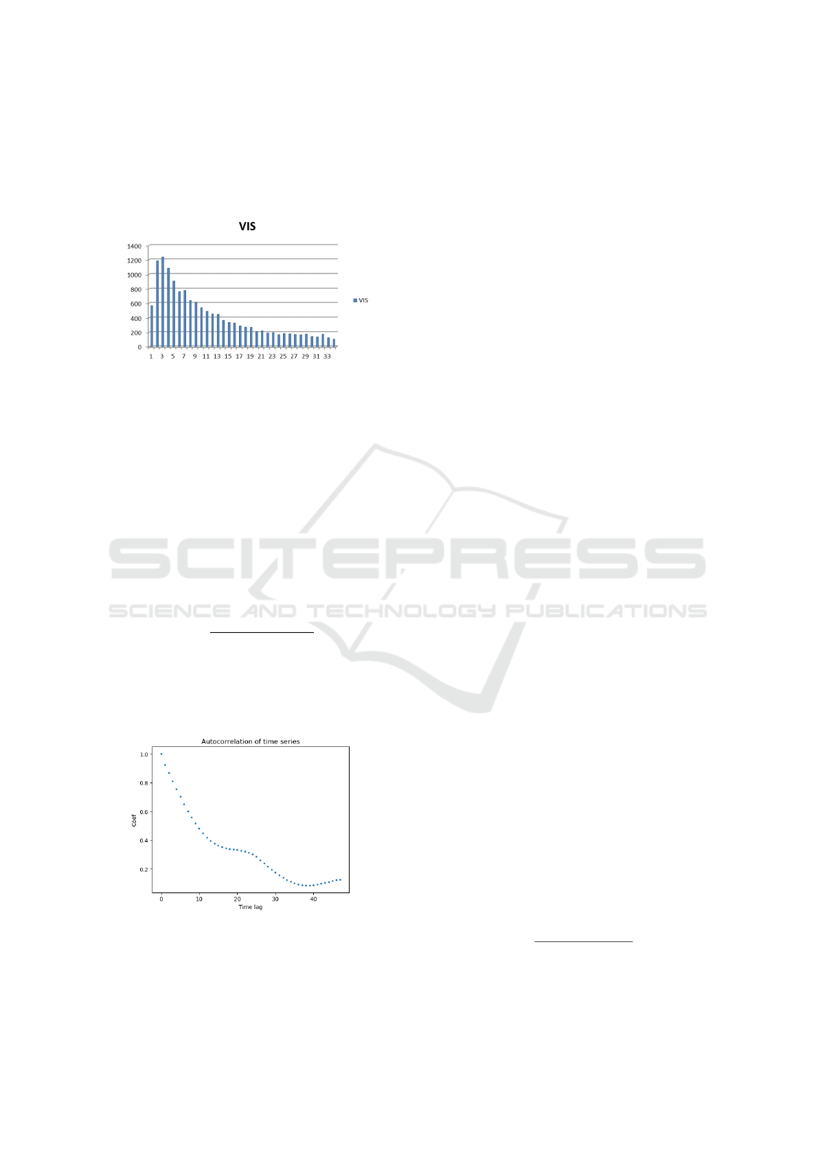
than 3,000 meters gradually decreases. For the low-

visibility data which we are most concerned with, the

amount of existing data is also small, which makes

it difﬁcult to obtain sufﬁcient training for these most

interesting situations.

Figure 2: Distribution of Visibility in Beijing Station.

2.2 Spatiotemporal Correlation

Analysis

The spatial correlation of visibility among the stati-

ons is measured by Pearson’s correlation coefﬁcient,

which is shown in Table 1. We can see that in most

cases the correlation coefﬁcient between S0 and other

stations is above 0.5.

We use the autocorrelation function to measure the

correlation among visibility in time series at Beijing

station. For time lag k, we calculate the autocorrela-

tion coefﬁcients with following formula:

Cov(L(t), L(t + k))

L(t)

L(t+k)

(1)

where L(t) and L(t + k) represent the meteorological

observation data of the same station with k time steps

difference. Cov(.) stands for covariance and σ stands

for standard deviation.

Figure 3: Autocorrelation coefﬁcient in Beijing Station.

The autocorrelation coefﬁcient of visibility in Bei-

jing station is shown in Figure 3. As the time lag

increases, the autocorrelation of time series shows a

clear downward trend, which agrees with the com-

mon sense that the closer events have greater inﬂu-

ence. From Figure 3 we can see that autocorrelation

is above 0.8 for visibility values within 3 hours, and

then drops rapidly until it reaches 0.4 for visibility be-

tween 12 hours. After that, autocorrelation slowly de-

creases, reaching about 0.3 at 24 hour. We ﬁnd that

the meteorological information after 24 hours is basi-

cally not related to the current stage. Therefore, we

decide to use the data of the past 24 hours as a single

input item for the model.

2.3 Fixing Missing Values

Due to failures of measure instruments and other dis-

turbances, there are often missing values in the obser-

vation data. The missing rate of all features is sum-

marized in Table 2. One way to handle the missing

data is to omit the missing values directly in time se-

ries prediction (Fan et al., 2017). However, compared

to other factors, the missing rate of PM10 and wind

direction is higher. For this part of data, if we neg-

lect the missing value directly, we may lose important

information. In this paper, we use the method of spa-

tially nearest neighbour interpolation to complement

the data, which almost does not affect the autocorre-

lation of time series itself, but supplement the infor-

mation by data from different sites.

Let L(t) = {x

,··· ,x

} be a sequence with

missing values. Each observation x

(i = 1, 2, · · · ,t)

has nine features. We traverse the time series in order

and mark the missing data, which will replaced by the

values from nearest neighbour. If there is a missing

data, select the next adjacent site to ﬁll the data. To

summarize, the missing values can be ﬁxed through

following steps.

Step1: Use Nearest Neighbour interpolation as a

replacement of a missing data and skip if a vacancy

still exists in the chosen site.

Step2: Remove used sites and repeat step 1 until

the data is completely ﬁlled

2.4 Data Normalization

Since the range of various meteorological elements is

different, we normalize all data to values between 0

and 1. In Table 3, we can see the statistical characte-

ristics of each meteorological element.

A feature x

is normalized as follows

− min(x

)

max(x

) − min(x

)

(2)

Through normalization, we can effectively avoid nu-

merical problems in gradient calculation. For itera-

ICAART 2019 - 11th International Conference on Agents and Artiﬁcial Intelligence

468

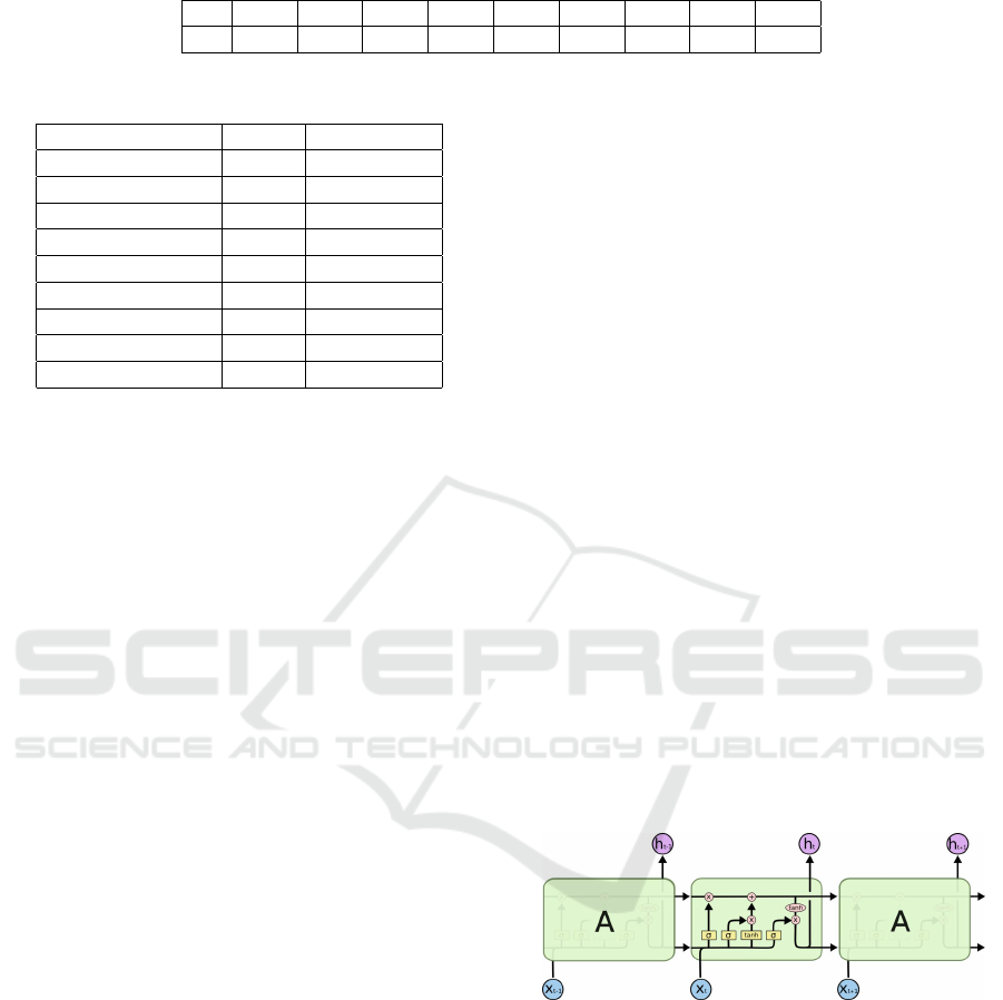
Table 1: Corr of visibility between stations.

L S1 S2 S3 S4 S5 S6 S7 S8 S9

S0 0.66 0.74 0.42 0.83 0.71 0.62 0.66 0.42 0.19

Table 2: Missing rate of measurement values.

Factor Unit Missing rate

PM10 ug/ml 1.72%

PM2.5 ug/ml 0.16%

Pressure hPa 0.03%

Temperature

◦

C 0.03%

Relative humidity % 0.03%

Precipitation mm 0.03%

Wind direction (

◦

) 3.78%

Wind speed m/s 0.03%

Visibility m 0.04%

tive algorithms in neural networks, normalized data

can also converge faster.

2.5 Data Conﬁguration

For time series prediction problems, the input and out-

put of the model have special forms (Bontempi et al.,

2012). Without loss of generality, we will summarize

the time series prediction model as follows

t+d

= f (x

t−1

,··· ,x

t−n+1

) + ε (3)

where {x

,··· ,x

t+d

} is time series data we al-

ready have and f is the model we build. ε is the irre-

ducible error. In equation (3), we use the data from

the past n time steps to predict the state after d time

steps.

Before building the model, we need to conﬁ-

gure the input and output. For the time series pre-

diction problem, our input is a matrix and the out-

put is a vector. More speciﬁcally, the time series

,··· ,x

t+d

} forms a [(t −n+1)∗n] input ma-

trix as in equation (4) and a [(t − n + 1) ∗ 1] output

vector as in equation (5)







t−1

··· x

t−n+1

t−1

t−2

··· x

t−n

n−1

··· x







(4)







t+d

t+d−1

n+d







(5)

where d is the time step we want to predict in the fu-

ture.

3 LSTM MODEL

In this section, we introduce the basic principles of the

LSTM model and describe resampling. At the end of

this section, we deﬁne the evaluation criteria of the

model.

3.1 LSTM

As it is known, RNN is sensitive to short-term in-

formation and insensitive to long-term information,

which is caused by the gradient vanishing problem. In

order to solve this problem, the LSTM model was pro-

posed in 1997 (Hochreiter and Schmidhuber, 1997)

and has been improved since (Greff et al., 2016).

Roughly speaking, LSTM model is a special RNN

neural network structure controlled by gates, which

is widely used in time series prediction. Figure 4 is

an illustration of LSTM.

The LSTM model has a chain structure which is

similar to the RNN model. The neurons in RNN are

replaced by memory blocks which have three units:

input gate,output gate and forget gate. The gate struc-

ture of LSTM solves the gradient vanishing problem,

thus enables the long-term dependence of time series.

Similar to RNN, the parameters of the LSTM

model are ﬁtted by back propagation through

time(BPTT).

Figure 4: LSTM.

3.2 Resampling

The resampling method can be traced back to the

randomization test proposed by Fisher in the 1930s

(Simon, 1992). According to the original resampling

idea, when the two sample sets were merged, there

should be no difference between the resampled statis-

tical indicators and the original sample statistical indi-

cators unless they came from different natural models

(Bi et al., 2009).

In recent years, resampling methods are gradually

being applied in the ﬁeld of machine learning, among

Visibility Forecast for Airport Operations by LSTM Neural Network

469

Table 3: Statistical characteristics of facors.

Factor Range Mean Std

PM10 [3,1000] 110.36 89.57

PM2.5 [1,1000] 81.88 75.16

Pressure [989.8,1037.5] 1011.82 10.12

Temperature [-9.9,38.2] 15.73 11.20

Relative humidity [5,98] 53.10 24.39

Precipitation [0,52.7] 0.08 0.99

Wind direction [0,360] 162.89 99.96

Wind speed [0,9.5] 2.03 1.32

Visibility [23,35000] 13454.64 11487.26

which bagging method and boosting method are po-

pular (James et al., 2013). In these methods, new data

sets are obtained by resampling, and these data sets

are applied to ensemble algorithm. In some cases, we

also verify the model with a random subset, which is

commonly known as cross-validation.

In this paper, we will use the resampling idea to

supplement the training set in the case of insufﬁcient

data volume. We obtain new data by sampling with

replacement. The new data are combined with the ori-

ginal data to supplement the training set.

3.3 Evalution Criterion

We use the Root Mean Squared Error (RMSE) to eva-

luate the model

RMSE =

∑

i=1

( ˆy

− yi)

(6)

where ˆy

is the predicted value and y

is the true value.

Consider the impact of low visibility to safety ope-

rations, we focus on low visibility forecast, which we

will evaluate separately. After the predicted results

are obtained, we will take out the data below 1600

meters and 800 meters and calculate their RMSE re-

spectively. These two dividing lines are the common

visibility standards for airports operations regarding

safe aircraft taking-off and landing.

4 EXPERIMENT AND ANALYSIS

In this section, we will introduce the detail of experi-

ments. First, we predict the visibility after one hour,

and improve forecast accuracy in low visibility situ-

ations by weighted RMSE. After that, we predict the

visibility after three hours. As the forecast time incre-

ases, the error becomes larger, and the result shows

clearly there is delay between the predicted and the

actual time series. We try to solve this problem by ad-

justing the structure of the model and by resampling.

4.1 One-hour Visibility Forecast

In this case, we build models for one-hour visibility

forecast with very simple neural network structure.

Since the prediction time is short and information be-

tween input and output is more correlated, the sim-

ple structure can reduce the model complexity and the

calculation time without suffering too much.

As described in Section 2.5, we select 24 hours

of meteorological information as input and the visibi-

lity for the next hour as output. For each set of inputs,

we select all nine meteorological elements as features,

and we also add the difference in visibility to provide

trend information for visibility changes in advance.

Therefore we have ten features in one set of data: tem-

perature, precipitation, pressure, wind speed, wind

direction, relative humidity, PM2.5, PM10, visibility

and difference value between visibilities.

We construct our model by a neural network with

two hidden layers. The ﬁrst hidden layer is the LSTM

layer containing 200 neurons and the second is the

fully connected layer with one neuron, as shown in

Figure 5. For other parameters, we choose the tanh

function as activation function and adam as optimizer.

In order to get better forecast for situation of low

visibility, we design a weighted RMSE (Eq.(7)) as

loss function. In the loss function, we add a hyperpa-

rameter α to adjust the weight of different data. The

weight e

−α∗y

is larger for lower visibility y

W RMSE =

∑

i=1

−α∗y

( ˆy

− yi)

(7)

Table 4 shows the RMSE for all test set becomes

larger when the value of α increases. RMSE is 4390

when α = 0, which means the weight for all error

term is 1, and increases to 5208 when α grows to

5. However, as the α increases, the RMSE of low

visibility part will ﬁrst decrease and then increase,

which is easy to understand since we give the error

term of low visibility part a higher weight. A furt-

her increase of α makes the weighted term in the loss

ICAART 2019 - 11th International Conference on Agents and Artiﬁcial Intelligence

470

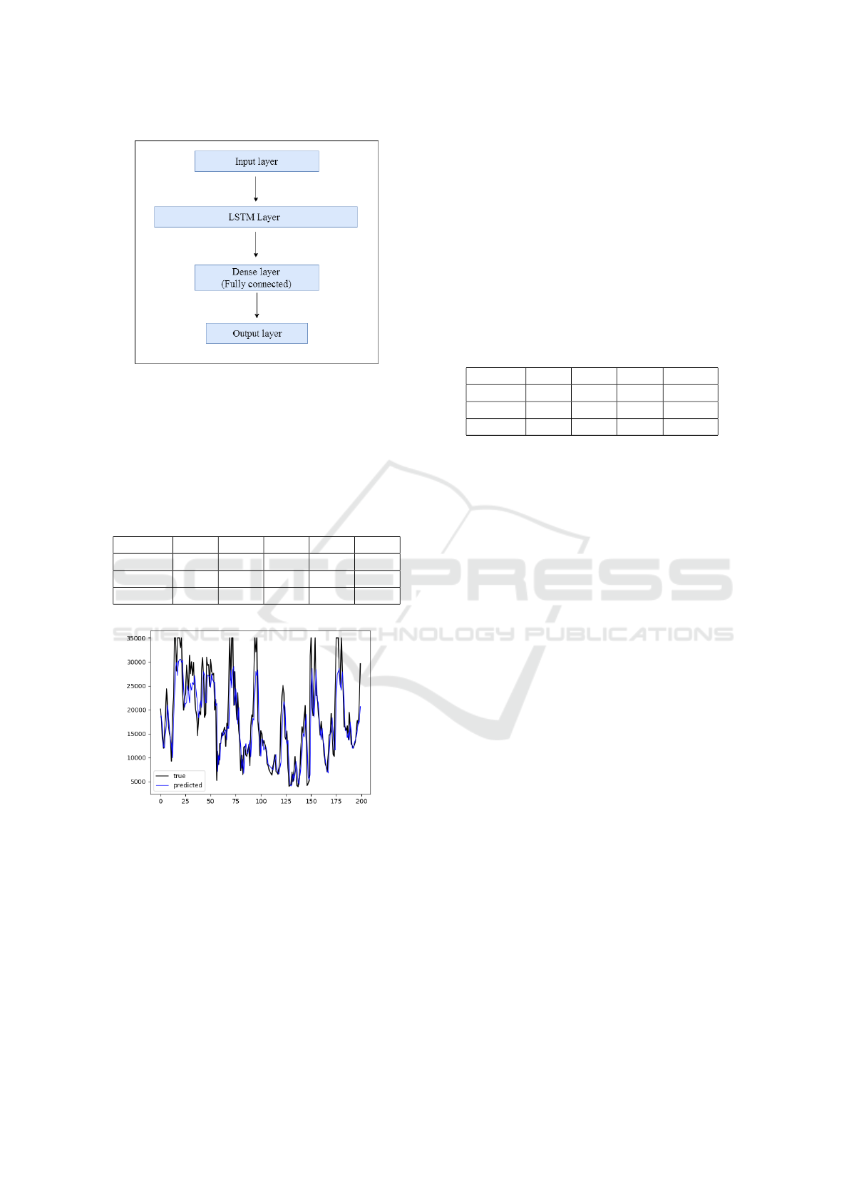
Figure 5: LSTM structure.

function (Eq.(7)) close to zero, and the model optimi-

zation stops. When α = 2, the RMSE of low visibility

part is minimal. The result of α = 2 is shown in Fi-

gure 6. The ﬁrst 200 time steps from the test set are

shown, where the blue line is the predicted value and

the black is the true value.

Table 4: RMSE by different α.

α 0 1 2 3 5

all data 4390 4572 4708 5107 5208

< 1600 1564 1118 933 1321 1373

< 800 1251 993 756 1233 1391

Figure 6: 1 hour visibility forecast with α = 2.

We can see that in Table 4 the weighted loss

function has a signiﬁcant improvement effect on the

forecast model. The improved model has higher pre-

diction accuracy for low visibility whereas the overall

prediction accuracy becomes worse, which is not the

focus in this speciﬁc application though. It can be

seen in Figure 6 that when α = 2, the overall trend

of the model’s prediction results is consistent with the

observation data.

In order to evaluate the performance of LSTM, we

compare the prediction results of LSTM model with

other commonly used forecast models in previous stu-

dies, namely, polynomial ﬁtting model (Fan et al.,

2016), regression tree model (Dietz et al., 2017) and

MLP model (Zhu et al., 2017). Polynomial ﬁtting is

used for the relationship between real-time elements,

and the latter two models are used for time series pre-

diction with similar data conﬁguration as in Section

2.5. In previous works mentioned above, limited by

the number of features used and models themselves,

these methods are usually used for short-term visibi-

lity prediction, such as one hour or even shorter. The

prediction results of the models in the following table.

Table 5: RMSE of different model.

RMSE Poly RF MLP LSTM

all data 6393 4432 4732 4708

< 1600 2113 1362 1517 933

< 800 2579 1811 2087 756

As can be seen from Table 5, compared with other

three methods, the overall error of the LSTM model

for visibility prediction has not been reduced, but the

prediction results for the low visibility part have been

signiﬁcantly improved, which is also the most rele-

vant in practical applications.

4.2 Three-hours Visibility Forecast

It is shown in the previous section that the LSTM mo-

del is effective for 1-hour visibility prediction. Re-

latively accurate predictions can be obtained with a

simple neural network structure. In the following,

we consider prediction of 3 hours with more complex

neural network structure, because the increase of pre-

diction time will lead to the loss of relevant informa-

tion in time series.

For the 3-hour visibility prediction model, we take

the same input dimension, which is the meteorologi-

cal data of the past 24 hours. Each set of data inclu-

des the ten elements. We change the complexity of

the model by adjusting the network structure. In the

previous section we use the structure with two hidden

layers, and now we will add more LSTM layers and

investigate the effects. In the experiment, we add one

LSTM layer each time, while each layer contains 200

neurons. For computational efﬁciency considerations,

we limit to add up to the model with four LSTM lay-

ers. Between multiple LSTM layers, we add dropout

to prevent overﬁtting. Before the output layer, we still

add a fully connected layer with one neuron.

In the experiments, we add more hidden layers

while keeping other parameters unchanged. We use

the weighted loss function with α = 2.

Visibility Forecast for Airport Operations by LSTM Neural Network

471

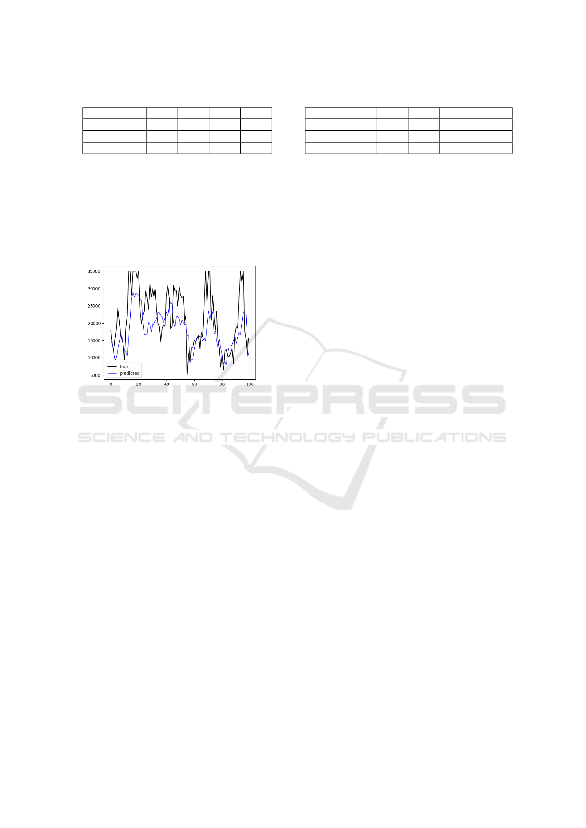
Table 6: RMSE by different number of layers.

LSTM layers 1 2 3 4

all data 7006 7013 7063 7710

< 1600 2149 1906 1685 1159

< 800 2702 2249 2159 1763

From Table 6 we can see that when the neural net-

work structure has fewer layers, the prediction results

are more accurate for the whole data. Neural network

structure with more layers obtains more accurate pre-

diction for low visibility situation. Figure 7 illustrates

the results of the 3-hour visibility forecast model with

only one LSTM layer, only the ﬁrst 100 time steps in

the test set is shown.

Figure 7: 3 hour visibility forecast with 1 LSTM layer.

Although the prediction accuracy of low visibi-

lity cases is improved by sacriﬁcing that for the high

visibility cases, Figure 7 shows there is a signiﬁ-

cant ”time delay” between the predicted result and

the actual value for 3-hour visibility forecast model.

By constructing a simple experiment with a periodic

function, we ﬁnd that this result is partly due to the

lack of data volume. Through experiments of trigono-

metric functions and other periodic functions that we

construct randomly, we ﬁnd that this phenomenon is

not only in the visibility prediction problem, but also

ubiquitous in the LSTM model applied to time series

problems, which can be solved when the amount of

data is sufﬁcient.

To solve this problem, we try to generate more

data by resampling. Speciﬁcally, after obtaining the

input matrix through data conﬁguration, sampling

with replacement is carried out by row, that is, res-

ampling by group. These data sets are added to the

input matrix after the resampling. Without loss of ge-

nerality, we choose the simplest neural network struc-

ture to study the resampling modeling. The results are

shown in Table 7.

After data conﬁguration, we randomly selected

5,000 to 15,000 groups of data as new data to supple-

ment the training set. It can be seen from the table that

Table 7: RMSE of resmapling model.

Added samples 0 5000 10000 15000

all data 7006 6824 6653 6844

< 1600 2149 1360 1628 1516

< 800 2702 1663 2291 2009

appropriate resampling can improve the model. When

the data volume of resampling is 5000, we can see

that RMSE is signiﬁcantly reduced. However, when

more data are added, the RMSE increases rather than

decreases, which is due to the problem of overﬁtting.

More speciﬁcally, beyond a certain point of adding

data via resampling, the loss function is still decreas-

ing, while the RMSE of the test set is increasing. In

summary, proper resampling can reduce errors in the

original model. However, constraint by the limited

amount of data, the ”time delay” problem cannot be

solved.

5 CONCLUSIONS

In this paper, we transform the traditional visibility

prediction problem into time series prediction pro-

blem, and predict the visibility by LSTM model.

Compared with previous studies mainly use simple

polynomial ﬁtting and MLP, the LSTM model per-

forms better in the overall trend and the accuracy. By

introducing a weighted loss function, we can improve

the accuracy of low visibility prediction. Speciﬁcally,

with appropriate hyperparameters, the RMSE of visi-

bility is reduced by 37% for cases of less than 1600

meters and by 21% for cases of less than 800 meters.

For short-term visibility prediction, our study shows

that the LSTM model can be used to aid airport opera-

tions in decision about suitability of take-off and lan-

ding of aircraft.

In the 3-hour visibility prediction model, we ﬁnd

that with complex LSTM structure, the overall error

of the model will become larger, but the RMSE of

the low visibility part will decrease, which is what we

hope to see. In predictions of many hours ahead(e,g.

6 or 8 hours), we encountered a systematic time delay

in LSTM forecast result. We investigated the causes

of this problem with a periodic function ampliﬁed by

a time dependent factor that we randomly construct, it

is shown that the LSTM model has a signiﬁcant time

delay for the prediction of multiple time steps when

the amount of data is insufﬁcient. This phenomenon

not only appears in the visibility prediction, but also

widely exists in time series prediction problems with

LSTM. We ﬁnd this is partly due to insufﬁcient me-

asurement data and try to solve it by resampling. In

our experiment, resampling can effectively reduce the

ICAART 2019 - 11th International Conference on Agents and Artiﬁcial Intelligence

472

error, but constraint by the limited amount of data the

”time delay” phenomenon is not completely elimina-

ted.

REFERENCES

Bi, H., Liang, H., and Wang, W. (2009). Resampling

method and machine learning. Journal of Computer,

32(5):862–877.

Bontempi, G., Taieb, S. B., and Le Borgne, Y.-A. (2012).

Machine learning strategies for time series forecas-

ting. In European Business Intelligence Summer

School, pages 62–77. Springer.

Clark, P. A., Harcourt, S. A., Macpherson, B., Mathison,

C. T., Cusack, S., and Naylor, M. (2008). Prediction of

visibility and aerosol within the operational met ofﬁce

uniﬁed model. i: Model formulation and variational

assimilation. Quarterly Journal of the Royal Meteo-

rological Society, 134(636):1801–1816.

Cortez, P., Rio, M., Rocha, M., and Sousa, P. (2006). Inter-

net trafﬁc forecasting using neural networks. In Neu-

ral Networks, 2006. IJCNN’06. International Joint

Conference on, pages 2635–2642. IEEE.

Dietterich, T. G. (2002). Machine learning for sequential

data: A review. In Joint IAPR International Works-

hops on Statistical Techniques in Pattern Recognition

(SPR) and Structural and Syntactic Pattern Recogni-

tion (SSPR), pages 15–30. Springer.

Dietz, S. J., Kneringer, P., Mayr, G. J., and Zeileis, A.

(2017). Forecasting low-visibility procedure states

with tree-based statistical methods. Pure and Applied

Geophysics, pages 1–14.

Fan, G., Ma, H., Zhang, X., and Liu, Y. (2016). Effects

of relative humidity and pm2.5 concentration on at-

mospheric visibility: a multi station comparative ana-

lysis based on hourly data. Journal of Meteorology,

74(6):959–973.

Fan, J., Li, Q., Hou, J., Feng, X., Karimian, H., and Lin,

S. (2017). A spatiotemporal prediction framework for

air pollution based on deep rnn. ISPRS Annals of the

Photogrammetry, Remote Sensing and Spatial Infor-

mation Sciences, 4:15.

Friedman, J., Hastie, T., and Tibshirani, R. (2001). The

elements of statistical learning. Springer series in sta-

tistics New York, NY, USA:.

Greff, K., Srivastava, R. K., Koutnik, J., Steunebrink, B. R.,

and Schmidhuber, J. (2016). Lstm: A search space

odyssey. IEEE Transactions on Neural Networks &

Learning Systems, 28(10):2222–2232.

Hochreiter, S. and Schmidhuber, J. (1997). Long short-term

memory. Neural Computation, 9(8):1735–1780.

James, G., Witten, D., Hastie, T., and Tibshirani, R. (2013).

An introduction to statistical learning, volume 112.

Springer.

Kurt, A. and Oktay, A. B. (2010). Forecasting air pollu-

tant indicator levels with geographic models 3 days in

advance using neural networks. Expert Systems with

Applications, 37(12):7986–7992.

Li, X., Peng, L., Yao, X., Cui, S., Hu, Y., You, C., and

Chi, T. (2017). Long short-term memory neural net-

work for air pollutant concentration predictions: Met-

hod development and evaluation. Environmental Pol-

lution, 231:997–1004.

Long, K., Li, C., Mao, X., and Hu, Y. (2017). Highway

foggy visibility prediction method. Journal of Xuzhou

Institute of Technology: Natural Sciences Edition, pa-

ges 31–37.

Minami, S. (2018). Predicting equity price with corporate

action events using lstm-rnn. Journal of Mathematical

Finance, 8(01):58.

Salman, A. G., Heryadi, Y., Abdurahman, E., and Suparta,

W. (2018). Weather forecasting using merged long

short-term memory model (lstm) and autoregressive

integrated moving average (arima) model. Journal of

Computer Science.

Simon, J. L. (1992). Resampling: the new statistics. arling-

ton, va: Resampling stats.

Song, M., Han, S., Zhang, M., Yao, Q., and Zhu, B. (2013).

Relationship between visibility and relative humidity

and pm10 and pm2.5 in tianjin. Journal of Meteoro-

logy and Environment, 29(2):34–41.

Wang, Q., Guo, Y., Yu, L., and Li, P. (2017). Eart-

hquake prediction based on spatio-temporal data mi-

ning: An LSTM network approach. IEEE Transacti-

ons on Emerging Topics in Computing, PP(99):1–1.

Wang, X., Han, J., Chen, J., Yan, W., and Yue, Y. (2016).

Variation characteristics of atmospheric visibility and

their relationship with relative humidity and particle

concentration in shijiazhuang of hebei. Journal of

Arid Meteorology, 34(4):648–655.

Yadav, A. P., Kumar, A., and Behera, L. (2013). Rnn ba-

sed solar radiation forecasting using adaptive learning

rate. In International Conference on Swarm, Evoluti-

onary, and Memetic Computing, pages 442–452.

Zhu, L., Zhu, G., Han, L., and Wang, N. (2017). The ap-

plication of deep learning in airport visibility forecast.

Atmospheric and Climate Sciences, 7(03):314.

Visibility Forecast for Airport Operations by LSTM Neural Network

473