Techniques for Automated Classiﬁcation and Segregation of Mobile

Mapping 3D Point Clouds

Johannes Wolf, Rico Richter and J

urgen D

ollner

Hasso Plattner Institute, Faculty of Digital Engineering, University of Potsdam, Germany

Keywords:

Mobile Mapping, 3D Point Cloud, Classiﬁcation, Semantics, Geodata.

Abstract:

We present an approach for the automated classiﬁcation and segregation of initially unordered and unstruc-

tured large 3D point clouds from mobile mapping scans. It derives disjoint point sub-clouds belonging to

general surface categories such as ground, building, and vegetation. It provides a semantics-based classiﬁ-

cation by identifying typical assets in road-like environments such as vehicles and post-like structures, e. g.,

road signs or lamps, which are relevant for many applications using mobile scans. We present an innovative

processing pipeline that allows for a semantic class detection for all points of a 3D point cloud in an automated

process based solely on topology information. Our approach uses adaptive segmentation techniques as well

as characteristic per-point attributes of the surface and the local point neighborhood. The techniques can be

efﬁciently implemented and can handle large city-wide scans with billions of points, while still being easily

adaptable to speciﬁc application domains and needs. The techniques can be used as base functional compo-

nents in applications and systems for, e. g., asset detection, road inspection, cadastre validation, and support

the automation of corresponding tasks. We have evaluated our techniques in a prototypical implementation on

three datasets with different characteristics and show their practicability for these representative use cases.

1 INTRODUCTION

Remote sensing technology (e. g., LiDAR) captures

our physical environment at different scales with high

precision using various carrier platforms (Schwarz,

2010); mobile mapping systems, for example, are

commonly used in the case of urban environments

and infrastructure networks. The resulting 3D point

clouds have established themselves as both efﬁ-

cient and effective discrete digital representations of

geospatial data (Vosselman et al., 2004) (“digital

twins”), used in a variety of application ﬁelds, e. g.,

for urban planning, disaster management (Biasion

et al., 2005), infrastructure monitoring and inspec-

tion (Teizer et al., 2005), facility management (Tang

et al., 2010), etc. Technically, they are stored as col-

lections of unstructured, unsorted, independent points

in three-dimensional space with optional attributes at-

tached to each point (Richter et al., 2013) (e. g., RGB

colors).

Besides aerial scans, mobile mapping techniques

have been established and used systems consist

“mainly of a moving platform, navigation sensors,

and mapping sensors” (Li, 1997); mobile carrier plat-

forms such as cars or trains are used to capture en-

tire infrastructure networks. Use cases include “street

view” services, urban planning, pothole detection,

risk analysis, e. g., for trees damaged in a storm, in-

frastructure monitoring, and inspection of clearance

areas along roads and railroads. Mobile mapping

scans can be used to, e. g., automatically construct

road networks, detect and monitor assets, or to an-

alyze road surfaces (Jaakkola et al., 2008), as well

as for the reconstruction of building fac¸ades. 3D

point clouds in combination with fac¸ade images can

be used to extract window structures and to construct

complete building models (Becker and Haala, 2007),

which is important for simulations.

Applications typically require only subsets of the

3D point cloud data, e. g., points representing struc-

tures of a speciﬁc semantic type, such as roads, build-

ings, or certain assets. A manual classiﬁcation is

neither viable nor practicable for complex objects or

large areas, e. g., entire cities, due to the massive

amount of data. Thus, automation represents a key

requirement for 3D point cloud classiﬁcation. From

a computational perspective, key challenges include

efﬁcient and adaptable classiﬁcation and segregation

algorithms for 3D point clouds taking into account

object-based and semantics-based criteria (Weinmann

Wolf, J., Richter, R. and Döllner, J.

Techniques for Automated Classiﬁcation and Segregation of Mobile Mapping 3D Point Clouds.

DOI: 10.5220/0007308802010208

In Proceedings of the 14th International Joint Conference on Computer Vision, Imaging and Computer Graphics Theor y and Applications (VISIGRAPP 2019), pages 201-208

ISBN: 978-989-758-354-4

201

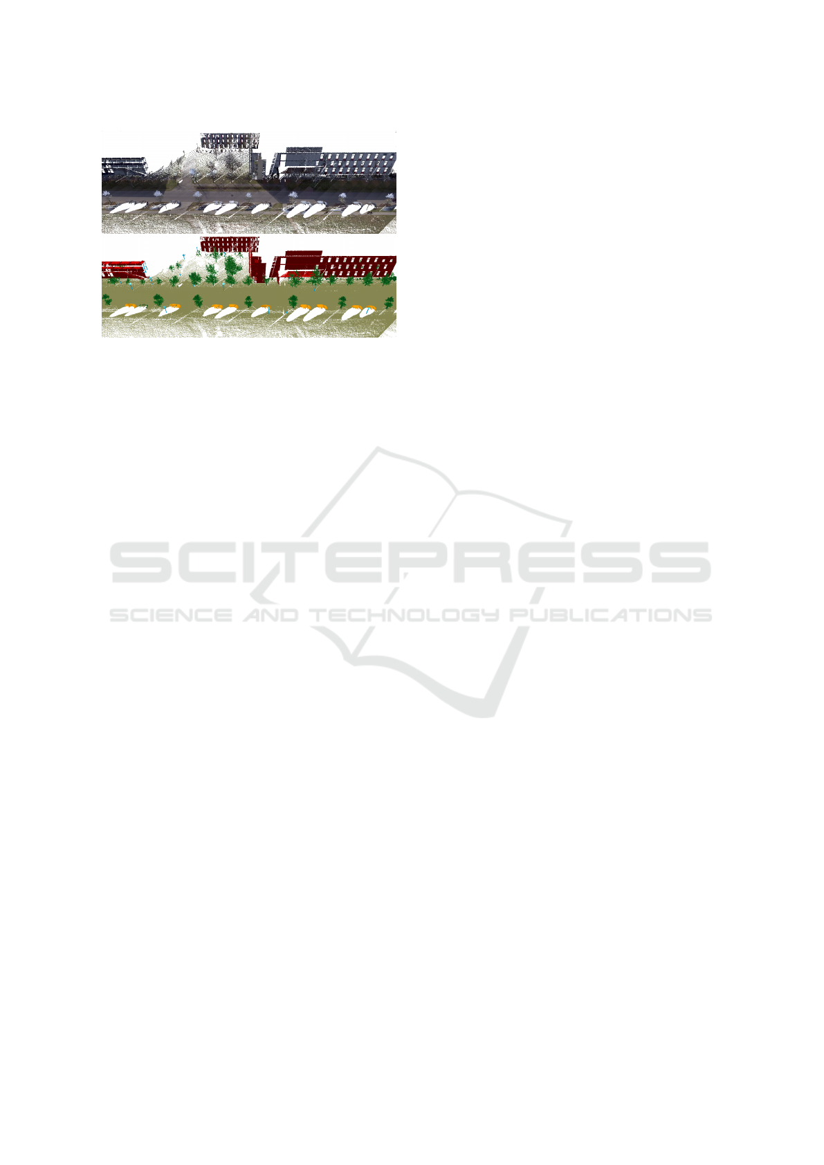
Figure 1: 3D point cloud of an urban area in RGB (top) and

segregated into sub-clouds colored by semantic class (bot-

tom). Ground: brown. Building: red. Vegetation: green.

Vehicle: orange. Post-like structure: blue.

et al., 2013).

Most classiﬁcation approaches for aerial data

implicitly assume an aerial perspective respectively

heightﬁeld-based point distributions (Charaniya et al.,

2004). Hence, they cannot be effectively applied

when it comes to mobile mapping scans that show

different geometric characteristics and point distribu-

tions. State-of-the-art approaches for classifying mo-

bile mapping scans often focus on detecting a single

semantic class. This paper concentrates on semantics-

based classiﬁcation based on the categories ground,

building, vegetation, vehicle and post-like structure

like lamps and signs, as shown in Figure 1.

In addition, we provide a scalable implementation

based on out-of-core concepts to cope with large 3D

point clouds (e. g., several terabytes of data) without

having to reduce density or precision in preprocess-

ing steps. All in all, this allows us automated classi-

ﬁcation and segregation via a processing pipeline that

consists of multiple steps. Step by step, we compute

and assign a semantic attribute to each point of the 3D

point cloud given as input data.

2 RELATED WORK

Niemeyer et al. (Niemeyer et al., 2012) distinguish

the ﬁve object classes “building”, “low vegetation”,

“tree”, “natural ground”, and “asphalt ground” in 3D

point clouds. Rutzinger et al. (Rutzinger et al., 2008)

separate vegetation from non-vegetation. While most

papers work on aerial 3D point clouds, classiﬁca-

tion has also been done for terrestrial scans, e. g., by

uchter et al. (N

uchter et al., 2006), who classify

points captured by a rescue robot driven indoors.

In general, separating vegetation from man-made

objects is a very essential step in the classiﬁcation

process as described by Yao and Fan (Yao and Fan,

2013) and Grilli et al. (Grilli et al., 2017). Yao and

Fan ﬁrst apply a segmentation on the 3D point cloud

and then classify trees within the data. Meinel and

Hecht (Meinel and Hecht, 2005) describe an approach

to ﬁnd areas with vegetation within mobile mapping

data. Rutzinger et al. (Rutzinger et al., 2011) analyze

tree parameters like crown diameter and stem height

for individual trees in 3D point clouds from mobile

mapping scans. They create 3D models for a “rep-

resentative and natural appearance of the individual

trees considering the real dimensions of stems and

tree crowns”.

In some cases the classiﬁcation is based on prob-

abilistic Markov networks (Triebel et al., 2006); an-

other approach analyzes the 3D point cloud’s topol-

ogy by speciﬁc characteristics like described by

Richter et al. (Richter et al., 2013). They do not re-

quire per-point attributes or any training data and base

their approach on an “iterative multi-pass processing

scheme, where each pass focuses on different topo-

logical features and considers already detected object

classes from previous passes”.

Besides buildings, vehicles, and vegetation,

cylinder-shaped structures (street lamps, signs, tree

stems) are found in most mobile mapping contexts.

A detection of lamps and road signs was done by

Lehtom

aki et al. (Lehtom

aki et al., 2010), who ex-

tracted “pole-like objects” from mobile mapping data.

Pu et al. (Pu et al., 2011) describe techniques to ﬁnd

posts and street signs and how these signs can be iden-

tiﬁed by their shapes. Fukanu and Masuda (Fukano

and Masuda, 2015) convert 3D point clouds into wire

frame models and use supervised machine learning

methods to detect utility poles, street lamps, trafﬁc

signals, and other post-like objects. Aijazi et al. (Ai-

jazi et al., 2013) use a voxelization approach for their

segmentation.

3 CLASSIFICATION METRICS

This paper introduces an approach for the classiﬁca-

tion and segregation of large 3D point clouds from

mobile mapping scans. Per-point metrics are com-

puted in a multipass process. The classiﬁcation tech-

niques are based on the analysis of additional per-

point attributes such as normal vector values and seg-

ment information. These attributes are computed for

all points of the point cloud prior to the classiﬁca-

tion. Adaptive segmentation is applied to the datasets,

which can then be segregated into sub-clouds based

on these metrics.

GRAPP 2019 - 14th International Conference on Computer Graphics Theory and Applications

202

3.1 Local Point Density

The local point density of a point is deﬁned as the

number of neighboring points in a certain volume

around the point divided by the size of this volume.

This value can be used to ﬁlter outliers and is used as

a metric during the classiﬁcation process.

3D point clouds from mobile mapping scans usu-

ally have hugely varying point densities depending on

the distance from the scanner to the target, causing the

need for an adaptive analysis.

An exact computation for local point density uses

a sphere with a speciﬁed radius around each point and

uses the number of points within this sphere divided

by its volume as the respective density value for the

point in the center of the sphere. However, to be able

to process large datasets in a short amount of time, an

approximate computation is used instead. The scene

gets separated into regular cube shaped voxels of a

deﬁned size and all points are assigned to the voxel

surrounding their position. Counting the number of

points in each voxel and dividing this number by the

voxel’s volume results in a density value for each

voxel. The density for a point is deﬁned based on

the number of points in surrounding voxels. This ap-

proach is less precise, but much faster than the indi-

vidual neighbor search using a sphere. As a trade-

off, a side length of, e. g, 0.33 meters for the voxels

has shown to deliver good results in different test data

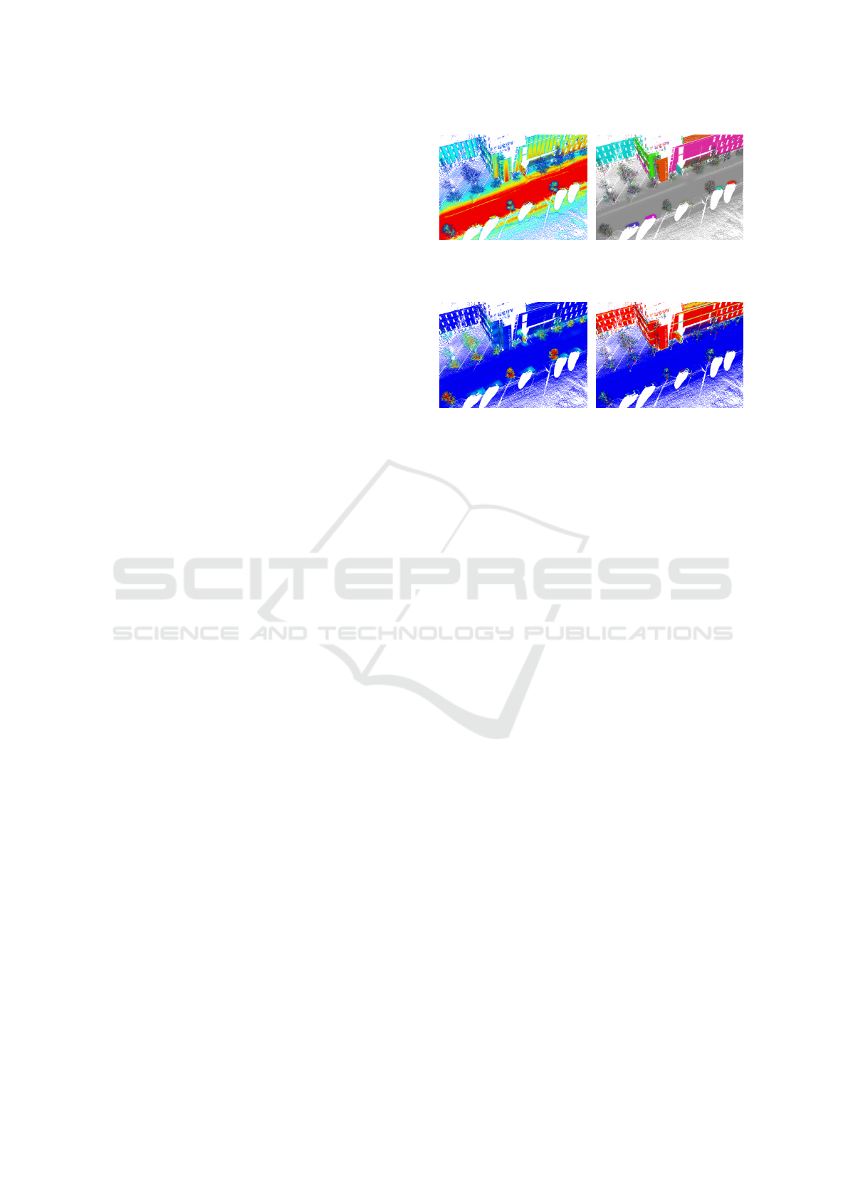
sets. Figure 2a shows a visualization of the local point

density.

The local point density can now be used to iden-

tify areas, where point information is too sparse to

make qualiﬁed statements about the semantic class of

a point. Only points with a density higher than a given

threshold of, e. g., 100 points per cubic meter are kept

in the classiﬁcation process.

3.2 Segment Size

A 3D point cloud can be segmented into disjoint

sub-clouds, each segment grouping together points

with similar properties based on different criteria, like

color, position, or normal vector orientation. In the

context of classiﬁcation, the segmentation creates in-

dividual segments for each object in the scanned en-

vironment. For example, all points of a vehicle will

optimally be grouped into one individual segment.

To achieve this segmentation, the position of points

is used as well as their normal vector orientation to

ﬁnd connected surfaces (Rabbani et al., 2006) during

a preprocessing step. Points belonging to the same

surface are assigned the same segment ID which is

stored as per-points attribute.

(a) Local point density. Blue

points have the lowest local

density, red points the high-

est.

(b) Segmentation. Points

with the same segment ID

have the same color.

points have the smallest seg-

ment density, red points the

highest.

(d) Verticality. Blue points

have the smallest verticality,

red points the highest.

Figure 2: Visualization of the different metrics.

Figure 2b shows the resulting segmentation. The

number of points belonging to the same segment is

used as a metric during the classiﬁcation process.

Building fac¸ades usually result in segments with a

large number of points due to their planar structure.

Vegetation on the other hand typically consists of

many segments with a small number of points.

3.3 Segment Density

The segment density of a point represents the number

of distinct segments that are positioned around this

point. It is used to identify regions with a large num-

ber of segments, which is usually the case for vege-

tation areas. As described before, the segmentation

aims to group points of the same object into one seg-

ment. Vegetation however is usually not segmented

into clearly separated objects by the used segmenta-

tion process because of its unstructured surfaces and

varying per-point normals.

The segment density can thus be used as a met-

ric to ﬁnd areas with many small segments to iden-

tify vegetation. For each part of the scene, e. g., each

voxel within a voxel grid, the number of segments

which have at least some of their corresponding points

in this voxel or one of the surrounding voxels, is

counted. Regions where this number is distinctively

higher than on average are usually vegetation areas.

Figure 2c shows a visualization of the segment den-

sity.

Techniques for Automated Classiﬁcation and Segregation of Mobile Mapping 3D Point Clouds

203

3.4 Verticality

The verticality value of a point describes the percent-

age of neighboring points forming a vertically ori-

ented surface. It is used to separate upright structures

like building fac¸ades from ground points and rounded

objects.

The verticality is deﬁned as the percentage of

neighboring points within the same voxel, which have

a horizontally oriented normal vector. All normal vec-

tors with an angle between 80 and 100 degrees to the

up vector are counted as horizontally oriented in our

implementation. Figure 2d shows a visualization of

the verticality metric.

Building fac¸ades have mostly horizontally facing

normal vectors, so they differ from their surroundings.

Ledges can have other orientations in their normal

vectors, but most parts of the fac¸ades can be identi-

ﬁed using this metric.

4 CLASSIFICATION APPROACH

The classiﬁcation uses the metrics described above

to determine the semantic class for each point of a

3D point cloud and to create the according segre-

gation into sub-clouds. A preprocessing step takes

place before the individual detection steps: First, all

points with a local point density signiﬁcantly lower

than the average are ﬁltered and marked as outliers.

All outliers are excluded from the following classiﬁ-

cation process. Second, individual normal vectors are

computed for each point and a segmentation based on

these normal vectors is applied to the dataset.

After the preprocessing step, points for each of the

semantic classes are segregated into the appropriate

sub-cloud.

4.1 Ground Detection

Ground points in mobile mapping data have simi-

lar characteristics as ground points in aerial data, al-

though point density and coverage differ. Existing

algorithms are based on the assumption that ground

points are usually the lowest points in a scanned area.

Tests show that an established technique for ground

detection in aerial data can be reused for the mobile

mapping classiﬁcation.

The algorithm divides the covered area into a reg-

ular two-dimensional grid. For each grid cell, the

minimum z-value of all points, which fall into this

cell, is stored. The result is a simpliﬁed terrain model.

This approach is originally based on the paper by

Meng et al. (Meng et al., 2009). It was reﬁned by

adding additional diagonal scan lines.

After the grid was initialized, scan lines are used

to ﬁnd all ground points of the 3D point cloud. These

scan lines move axis-aligned in positive and nega-

tive direction as well as diagonally through the grid.

The algorithm takes into account the slope found in

the different scanning directions and how the eleva-

tion differs between points and the minimum eleva-

tion in their local neighborhood. A majority voting

takes place, whether a point is a ground point from

the view of each of the scan lines or not. When more

scan lines ﬁnd the point to be a ground point than a

non-ground point, the semantic class attribute is set to

ground.

All following classiﬁcation steps analyze and op-

erate on the remaining points which are not part of the

ground points sub-cloud.

4.2 Building Detection

Buildings are typically the largest objects in mobile

mapping scans, their fac¸ades form the most charac-

teristic structures in the data and are processed next

in the classiﬁcation pipeline.

Buildings in typical urban areas mostly consist of

planar vertical faces. Windows and doors are also part

of the buildings as well as balconies and roof edges.

As planar faces usually result in large segments, all

segments with a small number of points are removed

from the analysis when searching for fac¸ade points

in the data. The remaining segments are ﬁltered by

their verticality. This metric was already described

in Section 3.4 and is used to ﬁnd vertically oriented

faces.

The verticality is a value between 0 (perfectly hor-

izontal) and 1 (perfectly vertical). Segments must at

least have a verticality of 0.6 to remain candidates

for the building classiﬁcation. All points of the seg-

ments fulﬁlling these criteria are classiﬁed as building

points. Not all points that actually belong to buildings

are part of these remaining segments. Many points

have been separated from the large segments and were

placed into smaller adjacent segments, which should

also be classiﬁed as building points. In a further step,

points that have not been classiﬁed yet can also get

the semantic class building, if they are located closely

to already classiﬁed building points.

All segments of the 3D point cloud that have not

already been classiﬁed are then checked one by one.

Figure 3 shows, in which step the points were classi-

ﬁed as building points.

Large vertical segments (blue points) were found

by the process described before. Points in large seg-

GRAPP 2019 - 14th International Conference on Computer Graphics Theory and Applications

204

Figure 3: Buildings in a 3D point cloud. Colors represent

the different steps in which the points were classiﬁed as

building points in the following order: blue, green, orange,

yellow.

ments that are within a 3m distance from the closest

segment already classiﬁed as building, also get classi-

ﬁed as building points (green points), mainly adding

balconies and window frames. The same is done for

all other segments regardless of their size, where at

least two thirds of their points are within a 1.5 m dis-

tance (orange points). This adds more window frames

and other small structures. To detect roofs, large seg-

ments that are located above building points are also

classiﬁed as building points (yellow points).

For performance reasons, the distances mentioned

above are measured by placing all found building

points into a voxel grid and computing the distance

to the closest voxel ﬁlled with building points for all

voxels in the grid. In this way, every voxel has an at-

tribute describing the distance to the closest “building

voxel”.

4.3 Vehicle Detection

Detecting vehicles is more difﬁcult than detecting

larger structures such as buildings. Where building

fac¸ades are very characteristic objects because of their

large planar surfaces, vehicles do not have such a

clear distinctive feature. Vehicles can have differ-

ent forms and sizes, but even when concerning buses,

the dimensions of vehicles are usually within certain

ranges, e. g., not wider than 2.5 meters. When ﬁl-

tering for vehicles, the segments must have dimen-

sions within these ranges and need to be located on

the ground. The distance to the ground for a seg-

ment is determined by the average vertical height dis-

tance to ground points which are located beneath and

close to this segment. This approach determines the

ground distance also for segments that do not have

any ground points directly beneath them, as it is often

the case for parking vehicles. Segments which are not

located on the ground can then be removed from the

search for vehicle segments, all remaining segments

are classiﬁed as vehicle, as well as small directly ad-

jacent segments.

4.4 Post Detection

For the post detection, all remaining unclassiﬁed

points are placed into a voxel grid. All voxels are ex-

amined and if they contain more than just a few single

points, they are marked as being “ﬁlled”, otherwise as

“empty”. The voxels are analyzed as if representing

sliced pillars: For each x-y coordinate combination

in the grid all voxels positioned upon each other are

analyzed from bottom to top. As long as the voxels

are ﬁlled, they are part of a potential post structure.

To prevent ﬁnding thin, outstretched structures, vox-

els that have neighboring ﬁlled voxels together reach-

ing more than a meter in a horizontal direction, are

not processed as potential post voxels.

Once an end during the vertical processing is

found, because a voxel is empty or fails the restric-

tion described above, the height of the collected po-

tential post voxels is calculated. If they are larger

than 1.5 meters, they are marked as post voxels and

all points within them are classiﬁed as post-like struc-

ture, as well as small directly adjacent segments.

4.5 Vegetation Detection

The segment density is a good indicator for vegeta-

tion, as described in Section 3.3. Smaller structures

within fac¸ades can also have a high density of very

small segments, so the approach works best when be-

ing applied after the building detection.

For the given segmentation, vegetation consists of

a large number of small segments. The segment den-

sity is computed for all voxels in the scene for all

segments that remained unclassiﬁed after the previ-

ous steps. Points in voxels with a segment density

much higher than average and with adjacent voxels

with a similar high segment density are classiﬁed as

vegetation points.

5 SYSTEM IMPLEMENTATION

The prototypic implementation, which is integrated

into an existing pipeline-based 3D point cloud re-

search framework using C++, Qt and the Point Cloud

Library (PCL), supports customized pipelines con-

sisting of conﬁgurable and connectable nodes via a

graphical user interface. Each node is either an in-

put node, output node, or processing node. Input and

output nodes are providing I/O functionality and can

read or write data ﬁles in multiple formats. Processing

nodes encapsulate computations for the processing of

3D point cloud data. The discussed mobile mapping

Techniques for Automated Classiﬁcation and Segregation of Mobile Mapping 3D Point Clouds

205

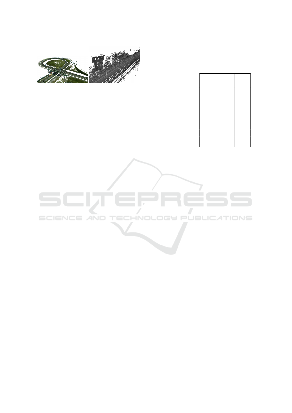
(a) Highway dataset colored

in captured RGB.

(b) Railroad dataset visual-

ized by grayscale intensity

values.

Figure 4: Screenshots of the second (a) and third (b) dataset.

classiﬁcation is available as a processing node and can

be reused in custom pipeline conﬁgurations.

Normal vector computation is done using the

PCL, approximating the surface at each point using

the covariance matrix of neighboring points and the

corresponding eigenvectors and eigenvalues (Hoppe

et al., 1992). A segmentation based on the surface

described by the computed normal vectors (Rabbani

et al., 2006) completes the preprocessing.

Our processing pipeline homogenizes the data and

scans are converted into one common coordinate sys-

tem. Large point clouds are tiled into data chunks,

which can be processed out-of-core.

A viewing application is also part of the frame-

work (Richter et al., 2015). It can load large 3D

point clouds and the visualization can be customized

based on any per point attribute. The visualization

allows for experimentally identifying appropriate pa-

rameters and thresholds for the classiﬁcation of a spe-

ciﬁc dataset.

6 EVALUATION

For this paper, three real-world datasets with differing

characteristics have been analyzed:

One dataset contains urban and suburban areas

with an average point density of 3 450 points/m

the road. Parked vehicles on the roads often cause

“shadowed” areas in this dataset, where no points

have been captured behind objects. Images from the

dataset are shown in ﬁgures 1, 2, and 3.

The second dataset was captured on an on-ramp

of a highway. It has an average road point density of

1 325 points/m

. This dataset does not contain other

vehicles and only low-growing vegetation.

A third dataset contains points captured by a train

on a railroad track. The average point density on the

track is 1 250 points/m

. The second and third dataset

are shown in Figure 4.

We have evaluated performance and accuracy of

our techniques using these mobile mapping scans.

Table 1: Performance measurements. Density values are

ground points per square meter. Time values are averaged

based on three test runs with identical parameters and those

for speciﬁc classiﬁcation steps are normalized per 1 000 000

points.

Urban area Highway Railroad

Data charac-

teristics

Number of points 18963 664 7373 756 6647 423

Number of segments 547324 146543 601152

Volume of bounding box 7190 580 m

2461 368 m

625000 m

Average density 3450 p/m

1325 p/m

1250 p/m

Maximum density 32124 p/m

2484 p/m

3494 p/m

Classiﬁcation

results

Number of points, thereof 18963 664 7373 756 6647 423

. . . Ground 56.7% 36.3% 67.6%

. . . Building 30.4% 8.7% 0.8%

. . . Vehicle 4.3% 0.0% 0.0%

. . . Post 0.3% 0.2% 0.4%

. . . Vegetation 4.2% 2.8% 23.6%

. . . Unclassiﬁed 4.0% 52.0% 7.6%

Processing times

per million points

Classiﬁcation, thereof 1.04s 5.55s 1.71s

. . . Preparation and Ground 0.25s 0.21s 0.22s

. . . Buildings 0.15s 0.29s 0.12s

. . . Vehicles 0.07s 0.05s 0.13s

. . . Posts 0.23s 4.69s 0.19s

. . . Vegetation 0.33s 0.29s 1.05s

Processing time for

complete point cloud 19.73s 40.93s 11.37s

The approach is able to handle large 3D point clouds

like city-wide scans in a both efﬁcient and robust way,

while still being easily adaptable to speciﬁc applica-

tion domains and needs. Especially when taking into

account how much time can be saved when exploring

a 3D point cloud with semantics information in con-

trast to an unclassiﬁed 3D point cloud, the presented

methods prove to be suitable for the classiﬁcation of

dense 3D point clouds from mobile mapping scans for

large areas.

In the urban test region all building points have

been correctly classiﬁed. All ground points in areas

with a sufﬁcient point density were found. 22 of 24

lamp posts and street signs were correctly detected

and 19 of the 22 existing vehicles were found, only

one group of points from a hedge was erroneously

classiﬁed as vehicle.

In an evaluation of the railroad dataset ground

points and building points were correctly identiﬁed.

All 15 signal and utility poles between the rails were

correctly detected.

However, some issues in the classiﬁed results ex-

ist. Especially bridges like the on-ramp of the high-

way pose a problem. The applied ground detection

does not detect the upper ground levels, so these re-

main unclassiﬁed. The dataset does not contain vehi-

cles or trees. This explains the high number of points

that remain unclassiﬁed in this dataset and a large

number of points is handed over from one classiﬁca-

tion step to the next, resulting in a long processing

time.

The classiﬁcation can efﬁciently be used for entire

cities, Table 1 shows the processing times for the three

exemplary datasets.

The complete mobile mapping dataset of the ur-

ban area consists of about 50 billion points, covers

GRAPP 2019 - 14th International Conference on Computer Graphics Theory and Applications

206

100km

, and uses about 920 GB of storage space.

Extrapolating the measured times for the test areas

shows that a classiﬁcation for the complete city takes

less than 15 hours for the complete dataset.

7 SUMMARY AND

CONCLUSIONS

Classifying and segregating 3D point clouds from

mobile mapping scans represent key functionality as

it provides semantics information and allows for efﬁ-

cient processing of large data sets. The implemen-

tation divides ground points from building fac¸ades

and vegetation; it is able to ﬁnd vehicles as well as

post-like structures like street lamps and sign posts.

Concepts for ground detection from the ﬁeld of aerial

point clouds can also be used in that framework. In

particular, the local point-density metrics turned out

to allow us to manage the greatly varying point den-

sity typical for mobile mapping scans and can be used

to ﬁlter areas unsuitable for classiﬁcation if the local

point-density falls under a given threshold.

Tests on different datasets show that the tech-

niques can be used to automatically and correctly

identify the semantic class points belong to, whereby

we obtained the best results for ground and build-

ings. Detecting vehicles as well as distinguishing

lamp posts from tree stems require a more detailed

analysis and highly depend on the quality of the ap-

plied segmentation.

Deﬁning the order of processing steps enables us

to select the most distinctive metrics of each semantic

class one at a time and, thereby, permits using the re-

sults of previous classiﬁcation steps. The processing

speed can be signiﬁcantly accelerated using a voxel

grid as spatial datastructure, i. e., the voxel-based met-

rics are used and their results can be applied to all

points in the respective voxel if approximate values

are sufﬁcient for the current use case.

The approach also allows for a computationally

fast exploration of points of a speciﬁc semantic sub-

cloud and supports ﬁltering options in viewing appli-

cations for detailed analysis of those objects the user

is interested in. In our test scenarios, the classiﬁcation

could analyze about 34 million points per minute.

In summary, the object-based and semantics-

based classiﬁcation and segregation techniques serve

as key components to process and manage large 3D

point clouds from mobile mapping scans, e. g., for

systems dedicated to asset detection, road inspection,

cadastre validation, or municipal tasks. Semantic

classiﬁcation offers a number of applications, e. g.,

using different 3D rendering techniques for each cat-

egory, and reduces the amount of data to be processed

for the respective category, e. g., by storing and man-

aging only those sub-clouds relevant to the applica-

tion’s purpose.

While the results of our study show that the de-

scribed classiﬁcation is already beneﬁcial and robust

for analyzing mobile mapping scans, the algorithms

could be further improved in multiple ways. Separat-

ing buildings from ground and vegetation is the most

important differentiation when segmenting 3D point

clouds. However, the more detailed the classiﬁca-

tion gets, the more use cases can be covered with the

data. The existing semantic classes could be used and

split into multiple subclasses: Introducing a more de-

tailed differentiation of ground points into road, curbs

and sidewalks would support the detection of cars and

lamp posts because assumptions about their locations

could be made. Buildings could be separated into

fac¸ades, doors and windows, balconies and the roof.

Finding doors in buildings would enable evaluations

about accessibility, especially in combination with the

analysis of curb stone heights.

Mobile mapping data often contains cars and

buses on the roads. A detection of cars was already

implemented, but it requires each car to be segmented

into only one large segment for best results. It would

make sense to improve the algorithm so that it can de-

tect adjacent segments, which together form a struc-

ture with certain characteristics.

Besides of ﬁltering points in areas with low den-

sity, points inside of buildings could also be detected.

If the location relative to already classiﬁed buildings

can be identiﬁed, this enables ﬁnding points that were

created because of reﬂective surfaces as well as points

that have been scanned through a building’s windows.

Those points could then be removed from the classi-

ﬁcation.

3D point clouds from mobile mapping scans could

be combined with data from aerial scans as well as

cadastral data, which would enrich the available data

pool. If data sets are combined taken at different

points in time, 4D point clouds result. Extending the

classiﬁcation and segmentation by a temporal com-

ponent would allow for new features. For exam-

ple, static objects like buildings would become dis-

tinguishable from mobile objects like cars, which are

not permanently ﬁxed to a speciﬁc position. 4D point

cloud enable analyses of areas that are occluded in

one scan, but might be available in another scan of the

same area or they could be used to analyze the same

region at different times of the year, showing changes

in foliation, vegetation growth, and the creation and

destruction of buildings.

Techniques for Automated Classiﬁcation and Segregation of Mobile Mapping 3D Point Clouds

207

REFERENCES

Aijazi, A. K., Checchin, P., and Trassoudaine, L. (2013).

Segmentation based classiﬁcation of 3d urban point

clouds: A super-voxel based approach with evalua-

tion. Remote Sensing, 5(4):1624–1650.

Becker, S. and Haala, N. (2007). Combined feature extrac-

tion for fac¸ade reconstruction. In Proceedings of the

ISPRS Workshop Laser Scanning, pages 241–247.

Biasion, A., Bornaz, L., and Rinaudo, F. (2005). Laser scan-

ning applications on disaster management. In Geo-

information for Disaster Management, pages 19–33.

Springer.

Charaniya, A. P., Manduchi, R., and Lodha, S. K. (2004).

Supervised parametric classiﬁcation of aerial lidar

data. In Conference on Computer Vision and Pattern

Recognition Workshop, 2004, pages 1–8. IEEE.

Fukano, K. and Masuda, H. (2015). Detection and clas-

siﬁcation of pole-like objects from mobile mapping

data. ISPRS Annals of Photogrammetry, Remote Sens-

ing and Spatial Information Sciences, 1:57–64.

Grilli, E., Menna, F., and Remondino, F. (2017). A review

of point clouds segmentation and classiﬁcation algo-

rithms. The International Archives of Photogramme-

try, Remote Sensing and Spatial Information Sciences,

42:339.

Hoppe, H., DeRose, T., Duchamp, T., McDonald, J., and

Stuetzle, W. (1992). Surface reconstruction from un-

organized points. Computer Graphics (SIGGRAPH

’92 Proceedings), 26(2):71–78.

Jaakkola, A., Hyypp

a, J., Hyypp

a, H., and Kukko, A.

(2008). Retrieval algorithms for road surface mod-

elling using laser-based mobile mapping. Sensors,

8:5238–5249.

Lehtom

aki, M., Jaakkola, A., Hyypp

a, J., Kukko, A., and

Kaartinen, H. (2010). Detection of vertical pole-

like objects in a road environment using vehicle-based

laser scanning data. Remote Sensing, 2(3):641–664.

Li, R. (1997). Mobile mapping: An emerging technology

for spatial data acquisition. Photogrammetric Engi-

neering and Remote Sensing, 63(9):1085–1092.

Meinel, G. and Hecht, R. (2005). Reconstruction of ur-

ban vegetation based on laser scanner data at leaf-off

aerial ﬂight times–ﬁrst results. Proceedings of the 31st

International Symposium on Remote Sensing of Envi-

ronment.

Meng, X., Wang, L., Silv

an-C

ardenas, J. L., and Currit, N.

(2009). A multi-directional ground ﬁltering algorithm

for airborne lidar. ISPRS Journal of Photogrammetry

and Remote Sensing, 64(1):117–124.

Niemeyer, J., Rottensteiner, F., and Soergel, U. (2012).

Conditional random ﬁelds for lidar point cloud classi-

ﬁcation in complex urban areas. ISPRS annals of the

photogrammetry, remote sensing and spatial informa-

tion sciences, 1(3):263–268.

uchter, A., Wulf, O., Lingemann, K., Hertzberg, J., Wag-

ner, B., and Surmann, H. (2006). 3d mapping with

semantic knowledge. In RoboCup 2005: Robot Soc-

cer World Cup IX, pages 335–346. Springer.

Pu, S., Rutzinger, M., Vosselman, G., and Elberink, S. O.

(2011). Recognizing basic structures from mobile

laser scanning data for road inventory studies. IS-

PRS Journal of Photogrammetry and Remote Sensing,

66(6):28–39.

Rabbani, T., Van Den Heuvel, F., and Vosselmann, G.

(2006). Segmentation of point clouds using smooth-

ness constraint. International Archives of Photogram-

metry, Remote Sensing and Spatial Information Sci-

ences, 36(5):248–253.

Richter, R., Behrens, M., and D

ollner, J. (2013). Object

class segmentation of massive 3d point clouds of ur-

ban areas using point cloud topology. International

Journal of Remote Sensing, 34(23):8408–8424.

Richter, R., Discher, S., and D

ollner, J. (2015). Out-of-

core visualization of classiﬁed 3d point clouds. In 3D

Geoinformation Science: The Selected Papers of the

3D GeoInfo 2014, pages 227–242. Cham: Springer

International Publishing.

Rutzinger, M., H

oﬂe, B., Hollaus, M., and Pfeifer, N.

(2008). Object-based point cloud analysis of full-

waveform airborne laser scanning data for urban veg-

etation classiﬁcation. Sensors, 8:4505–4528.

Rutzinger, M., Pratihast, A. K., Oude Elberink, S. J., and

Vosselman, G. (2011). Tree modelling from mo-

bile laser scanning data-sets. The Photogrammetric

Record, 26(135):361–372.

Schwarz, B. (2010). Lidar: Mapping the world in 3d. Na-

ture Photonics, 4(7):429.

Tang, P., Huber, D., Akinci, B., Lipman, R., and Lytle, A.

(2010). Automatic reconstruction of as-built building

information models from laser-scanned point clouds:

A review of related techniques. Automation in con-

struction, 19(7):829–843.

Teizer, J., Kim, C., Haas, C., Liapi, K., and Caldas, C.

(2005). Framework for real-time three-dimensional

modeling of infrastructure. Transportation Research

Record: Journal of the Transportation Research

Board, 1913:177–186.

Triebel, R., Kersting, K., and Burgard, W. (2006). Robust

3d scan point classiﬁcation using associative markov

networks. In Robotics and Automation, 2006. ICRA

2006. Proceedings 2006 IEEE International Confer-

ence on, pages 2603–2608. IEEE.

Vosselman, G., Gorte, B. G., Sithole, G., and Rabbani,

T. (2004). Recognising structure in laser scanner

point clouds. International archives of photogramme-

try, remote sensing and spatial information sciences,

46(8):33–38.

Weinmann, M., Jutzi, B., and Mallet, C. (2013). Feature rel-

evance assessment for the semantic interpretation of

3d point cloud data. ISPRS Annals of the Photogram-

metry, Remote Sensing and Spatial Information Sci-

ences, II-5/W2:313–318.

Yao, W. and Fan, H. (2013). Automated detection of 3d

individual trees along urban road corridors by mo-

bile laser scanning systems. In Proceedings of Inter-

national Symposium on Mobile Mapping Technology

(MMT), Tainan City, Taiwan, volume 13.

GRAPP 2019 - 14th International Conference on Computer Graphics Theory and Applications

208