Gap Distributions for Analysing Buyer Behaviour in Agent-based
Simulation
Andreas Ahrens
1
, Ojaras Purvinis
2
and Jelena Zaˇsˇcerinska
3
1
Hochschule Wismar, University of Technology, Business and Design, Wismar, Germany
2
Kaunas University of Technology, Kaunas, Lithuania
3
Centre for Education and Innovation Research, Riga, Latvia
Keywords:
Buyers’ Burstiness, Gap Processes, Binary Customer Behaviour, Exponential Distribution, Weibull Distribu-
tion, Wilhelm Distribution, Agent-based Simulation.
Abstract:
Simulation models allow predicting the development of real situations in various technical, business and so-
cial systems. However, many real situations in business environment are of bursty nature. Buyers often appear
concentrated or, in other words, bursty. Different approaches for analysing buyers’ behaviour have been de-
veloped. One of these approaches focuses on analysis of gaps between buyers, and the buyers’ scenario is
completely described by the sequence of gaps. The present research is interdisciplinary, namely telecommuni-
cations and business management. The methodology of the present contribution is built on adaptation of gap
distribution functions from data transmission theory in telecommunications to bursty business process in busi-
ness management. The aim of the paper is to demonstrate inter-connections between different gap distribution
functions such as Weibull, Exponential and Wilhelm as well as to compare different gap distribution functions
for their suitability when analysing bursty processes. Furthermore, this contribution provides the mathematical
description of gap processes. The comparison results of different gap distribution functions are presented. The
theoretical results are confirmed by practical implementation in agent-based simulation environment.
1 INTRODUCTION
Phenomenon’s simulation or, in other words, imita-
tion of a situation or process, allows predicting the
development of real situations in various technical,
business and social systems. Many real situations in
business environment are of bursty nature as shown
in telecommunication systems by Gilbert and Elliot
in the 1960s (Gilbert, 1960; Elliott, 1963). Contem-
porary computers and information and communica-
tions technology (ICT) facilitate phenomenon simu-
lation. When the mathematics is intractable, agent-
based simulation provides an efficient solution to sim-
ulate the bursty process of buying by taking decisions
of individual buyers, so called agents, into account
(Axelrod, 2006; Albanese, 2006; Tesfatsion, 2006).
Thus, in business process, agent-based simulation as-
sists in analysing buyers’ behaviour.
Different approaches for analysing buyers’ be-
haviour have been developed. One of these ap-
proaches focuses on analysis of gaps between buyers,
and the buyers’ scenario is completely described by
the sequence of gaps. However, in many situations,
buyers appear concentrated or, in other words, bursty.
Bursty processes are described by gap distributions
in data transmission theory in such a research field
as telecommunications. In such scenarios the classi-
cal Bernoulli model, also known as memoryless sce-
nario in data transmission theory, cannot be applied.
Mostly the Weibull gap distribution is usedto describe
bursty processes. Unfortunately, the parameters of
the Weibull gap distribution are notdirectly connected
with the process of buying.
A promising approach was formulated by Wil-
helm. Wilhelm described the distribution of bit-errors
(i.e. gaps between bit-errors) in data transmission
by defining a bit-error probability as well as a bit-
error concentration (Wilhelm, 1976). The Wilhelm
approachwas adapted by Ahrens to the bursty process
of buying by defining a buyer probability as well as a
buyer concentration (Ahrens et al., 2015; Ahrens and
Zaˇsˇcerinska, 2016). Both gap distribution functions,
namely Weibull as well as Wilhelm, can be applied
to describe bursty and non-bursty business processes.
Whereas the Bernoulli approach is well established in
statistical theory, in this paper we are going to show
Ahrens, A., Purvinis, O. and Zaš
ˇ
cerinska, J.
Gap Distributions for Analysing Buyer Behaviour in Agent-based Simulation.
DOI: 10.5220/0007308900230029
In Proceedings of the 8th International Conference on Sensor Networks (SENSORNETS 2019), pages 23-29
ISBN: 978-989-758-355-1
Copyright
c
 2019 by SCITEPRESS – Science and Technology Publications, Lda. All rights reserved
23

that the Wilhelm gap distribution function is an ex-
tension of the Bernoulli model (the same as for the
Weibull gap distribution).
The present research is interdisciplinary, namely
telecommunications and business management. The
methodology of the present contribution is built on
adaptation of gap distribution functions from data
transmission theory in telecommunications to bursty
business process in business management.
The novelty of this paper is the demonstration of
inter-connections between different distribution func-
tions as well as a comparison of different distribution
functions for their suitability when analysing bursty
processes. The paper provides the mathematical de-
scription of gap process and presents the comparison
results of different gap distribution functions. Practi-
cal implementation in agent-based simulation is used
to confirm the theoretical results.
The remaining part of this paper is structured as
follows: In section 2 the mathematical description of
gap processes is presented. In section 3 the proba-
bility of arbitrarily buyer’s patterns is demonstrated.
The comparison results of different gap distribution
functions are shown in section 4. Finally, the practical
implementationin agent-based simulation is shown in
section 5. Some concluding remarks are given in sec-
tion 6.
2 MATHEMATICAL
DESCRIPTION OF GAP
PROCESSES
Bursty buyer processes can be defined by gaps be-
tween consecutive buyers as highlighted in Fig. 1 and
2.
block interval n
buyer
sequence of people
visitor
Figure 1: Buyer processes defined by gaps between consec-
utive buyers.
- x - - x - - x - - - x x - - - - x -
2 2 3 40
Figure 2: Definition of gaps between consecutive buyers (a
buyer (represented by ”x”) within a sequence of non-buying
visitors (represented by ”-”)).
Frequently used and well-suited practical approx-
imations are provided, if the model is based on the in-
dependence of gap intervals. The gap distribution in-
dicates the probability that a gap X between two buy-
ers is greater than or at least equal to a given number
k, i. e.
u(k) = P(X ≥ k) (1)
as well as the gap density function v(k) defining the
probability that a gap X between two buyers is equal
to a given number k, i. e.
v(k) = P(X = k) . (2)
Models that are based on the independence of gap in-
tervals are completely described by the gap density
or the gap distribution, respectively. The assumption
that successive gaps are statistically independent is
regarded as a good practical approximation. Mod-
els with these requirements are described as regenera-
tive models in the literature (Wilhelm, 1976; Ahrens,
2000). Several gap distribution functions u(k) are
shown in Table 1. Whereas the Exponential distribu-
tion function is described by one parameter, Wilhelm
distribution as well as Weibull distribution are defined
by two parameters.
Table 1: Several gap distribution functions.
Type Distribution u(k)
Exponential e
−β
e
k
Weibull e
−(β
w
k)
α
w
Wilhelm ((k+ 1)
α
− k
α
) ·e
−β·k
When taking the gap distribution defined by Wil-
helm into account the following expression was iden-
tified
u(k) = ((k + 1)
α
− k
α
) · e
−β·k
0 ≤ k < ∞ (3)
with
lim
k→∞
e
−β·k
= 0 β > 0 (4)
and
β ≈ p
e
1/α
. (5)
Here, the business process, i.e. the buyers’ character-
istics, is modelled by two parameters, namely visitor
probability to buy (also referred as the buyers’ proba-
bility) p
e
and the buyers’ concentration (1− α). Typ-
ical values for the buyer concentration are (1−α) = 0
for the memoryless buyer scenario (also known as the
Bernoulli scenario), i. e. the buyers appear indepen-
dently distributed and 0 < (1− α) ≤ 0.5 for a bursty
buyer scenario. Assuming that the buyers appear in-
dependently form each other, i.e. (1 − α) = 0, the
buyers’ gap distribution function u(k) defined by Wil-
helm simplifies to
u(k) = e
−p
e
·k
= (e
−p
e
)
k
. (6)
SENSORNETS 2019 - 8th International Conference on Sensor Networks
24

Taking the Taylor series of the exponential function
e
−x
for small x into account, the function e
−x
can be
re-written as
e
−x
= 1− x+
x
2
2
−
x
3
6
+
x
4
24
+ · ·· (7)
and approximated by
e
−x
≈ 1− x (8)
for small x. Finally, the buyers’ gap distribution func-
tion u(k), defined in (3), results for small p
e
in
u(k) = P(X ≥ k) = (1 − p
e
)
k
=
p
k
e
. (9)
The parameter
p
e
described the probability of non-
buying and can be defined as
p
e
=
Number of Visitors - Number of Buyers
Number of Visitors
.
(10)
It should be noted that equation (9) is well-known
in probability theory for the product of independent
events and is valid for any p
e
. Obtaining equation
(9) testifies the correctness of the equality (3) for the
memoryless buyer scenario.
The probability of a non-buying visitor is given by
p
e
= (1− p
e
). Finally, the probability u(k) = P(X ≥
k) that X ≥ k consecutive visitors are non-buying vis-
itors results in
u(k) =
p
k
e
= (1− p
e
)
k
. (11)
Re-writing of u(k) leads to the buyers’ gap density
function v(k), i. e.
v(k) = P(X = k) , (12)
which describes the probability of a gap X equal to k.
The buyers’ gap density function v(k) can be calcu-
lated as follows
u(k) = v(k) + v(k+ 1) + v(k+ 2) + ·· ·
u(k+ 1) = v(k+ 1) + v(k+ 2) + ··· .
By calculating the difference between u(k) and
u(k + 1) the buyers’ gap density function v(k) =
P(X = k) can be obtained
v(k) = u(k) − u(k + 1) (13)
and results for the memoryless buying process with
(9) in
v(k) =
p
k
e
− p
k+1
e
= p
k
e
· (1− p
e
) (14)
and can be simplified as
v(k) = (1− p
e
)
k
· (1− (1− p
e
)) = (1− p
e
)
k
· p
e
.
(15)
The probability that after a buyer in the distance of
k = 0 another buyer appears results in
v(0) = p
e
(16)
and is solely defined by the buyer probability p
e
as
expected for the memoryless buyer scenario. In sit-
uations with bursty buyers, the probability v(0) in-
creased as highlighted in Fig. 3
0 2 4 6 8 10
10
−2
10
−1
10
0
v(k) →
n →
(1 − α) = 0.0
(1 − α) = 0.2
(1 − α) = 0.5
Figure 3: Buyers’ gap density function v(k) for different
parameters of the (1 − α) at a buyer’s probability of p
e
=
10
−2
.
3 STATISTICAL ANALYSIS OF
ARBITRARILY BUYERS’
PATTERNS
In this section, the proof is given that the beforehand
defined functions u(k) and v(k), introduced by Wil-
helm, can be used to calculate the probability of ar-
bitrarily buyer pattern with e buyers within an inter-
val of n visitors. Let us denote the number of pattern
with K
n,e
and start with the memoryless buyer sce-
nario with (1 − α) = 0. Analysing a pattern E of n
visitors with e buyers, total number of pattern within
an interval n is given by
K
n,e
=

n
e

=
n!
e!(n− e)!
. (17)
Here it is worth noting that when analysing the mem-
oryless buyer scenario all pattern E within an interval
of n visitors with e buyers appear with the same prob-
ability.
block interval
n = 7
buyer
with p
e
position
1 2
3
4
5 6
7
u(2)
u(4)
Figure 4: Calculation of the probability P
E
(7,1) of a pattern
E within an interval of n = 7 visitors with e = 1 buyer at the
position n
1
= 3.
According to Fig. 4, the probability P
E
(7,1) of such
a pattern E within an interval of n = 7 visitors with
Gap Distributions for Analysing Buyer Behaviour in Agent-based Simulation
25

e = 1 buyer results in
P
E
(7,1) = p
e
· u(2) · u(4) . (18)
The term p
e
· u(2) defines the probability that there
will be a buyer before the considered interval fol-
lowed by a gap of at least two visitors. With
u(k) = (1− p
e
)
k
=
p
k
e
. (19)
the probability P
E
(7,1) can be expressed for the con-
sidered pattern and the memoryless buyer scenario as
P
E
(7,1) = p
e
·
p
2
e
· p
4
e
= p
e
· p
6
e
, (20)
indicating that six non-buying visitors within an inter-
val of n = 7 visitors appear. Here the position of the
buyer is not of any interest, as the pattern depicted in
Fig. 5 results in the same probability for P
E
(7,1).
Taking two buyers within an interval of n visitors
into consideration as exemplary depicted in Fig. 6, the
probability P
E
(7,2) of such a pattern E within an in-
terval of n = 7 visitors results in
P
E
(7,2) = p
e
· u(2) · v(1) · u(2) . (21)
With
u(k) = (1 − p
e
)
k
=
p
k
e
(22)
and
v(k) = (1− p
e
)
k
· p
e
=
p
k
e
· p
e
(23)
the probability P
E
(7,2) can be expressed for the
memoryless buyer scenario as
P
E
(7,2) = p
e
· p
2
e
· p
e
· p
e
· p
2
e
= p
2
e
· p
5
e
(24)
indicating that five non-buying visitors within an in-
terval of n = 7 visitors with 2 buyers appear.
On the other hand, 2 buyers between 7 visitors
may appear in another sequence.
It yields from (17) that the total number of such
combinations (pattern) equals to
K
7,2
=

7
2

=
7!
2!(7− 2)!
= 21 . (25)
Therefore, the probability of 2 buyers between 7 visi-
tors of all patterns is given by the Bernoulli formula
P(7,2) = K
7,2
· P
E
(7,2) =
7!
2!(7− 2)!
· p
2
e
·
p
5
e
. (26)
block interval
n = 7
buyer
with p
e
position
1 2
3
4
5 6
7
u(3)
u(3)
Figure 5: Calculation of the probability P
E
(7,1)) of a pat-
tern E within an interval of n = 7 visitors with e = 1 buyer
at the position n
1
= 4.
block interval
n = 7
buyer
with p
e
position
1 2
3
4
5 6
7
u(2) v(1)
u(2)
Figure 6: Calculation of the probability P
E
(7,1) of a pattern
E within an interval of n = 7 visitors with e = 2 buyers at
the position n
1
= 3 and n
2
= 5.
Therefore, for the memoryless channel it can be
shown that the obtained results coincide with the
Bernoulli model.
Having more than 2 buyers within an interval of
n visitors, the probability P
E
(n,e) of a pattern E in
an interval of n visitors with e buyers at the positions
n
1
,n
2
,· ·· , n
e
can be obtained as
P
E
(n,e) = p
e
· u(n
1
− 1)· u(n−n
e
) ·
e
∏
ν=2
v(n
ν
− n
ν−1
− 1) .
(27)
The ith pattern (with 1 ≤ i ≤ K
n,e
) is determined by
the buyers’ position n
1
,n
2
,· ·· , n
e
.
Fig. 7 illustrates the calculation of the probability
P
E
(7,3) of a pattern E within an interval of n = 7
visitors. Here, the e = 3 buyers are at the positions
n
1
= 3, n
2
= 4 and n
3
= 6. The probability P
E
(7,3)
of such a pattern E within an interval of n = 7 visitors
is given by
P
E
(7,3) = p
e
· u(2) · v(0) · v(1) · u(1) . (28)
With
u(k) =
p
k
e
(29)
and
v(k) =
p
k
e
· p
e
(30)
the probability P
E
(7,3) can be expressed for the
memoryless buyer scenario as
P
E
(7,3) ≈ p
e
·
p
2
e
· p
e
· p
e
· p
e
· p
e
= p
3
e
· p
4
e
. (31)
block interval
n = 7
buyer
with p
e
position
1 2
3
4
5 6
7
u(2) v(0) v(1) u(1)
Figure 7: Calculation of the probability P
E
(7,3) of a pattern
E within an interval of n = 7 visitors with e = 3 buyers at
the positions n
1
= 3, n
2
= 4 and n
3
= 6.
SENSORNETS 2019 - 8th International Conference on Sensor Networks
26

Taking the total number of such combinations
(pattern) such as
K
7,3
=

7
3

=
7!
3!(7− 4)!
= 35 (32)
into account, the probabilityof 3 buyers in a sequence
of 7 visitors is given by the Bernoulli formula
P(7,3) = K
7,3
·P
E
(7,3) =
7!
3!(7− 3)!
· p
3
e
·
p
4
e
. (33)
Analysing the memoryless buyer scenario, the
probability P
E
(n,e) can be written as
P
E
(n,e) ≈= p
e
e
·
p
n−e
e
(34)
and is independent of the individual pattern when
analysing the memoryless buyer scenario where each
pattern E appears with the same probability.
4 COMPARISON OF GAP
DISTRIBUTIONS
In this section the interconnections of Exponential,
Weibull and Wilhelm distribution are to be shown. It
is assumed that the given buyers’ characteristic under-
goes the Wilhelm distribution with given parameters
p
e
and (1− α).
Table 2 and 3 show the resulting estimation errors
for p
e
= 10
−2
. As quality parameter for the approx-
imation between the given Wilhelm gap interval dis-
tribution u
Wilhelm
(k) and the investigated distribution
function u(k) (Exponential, Weibull) the mean square
error
MSE
min
=
k
max
−1
∑
k=0
|u(k) − u
Wilhelm
(k)|
2
(35)
is used and minimized when using least-square opti-
mization. The parameter k
max
specifies the maximum
gap length to be considered.
Tab. 2 shows the obtained results when using
an Exponential gap distribution instead of the Wil-
helm distribution. As the Exponentialgap distribution
equals the Wilhelm distribution for the memoryless
(non-bursty) buyer scenario, a perfect mapping can be
achieved. With increasing buyers’ concentration, the
gap between the Wilhelm and Exponential gap distri-
bution becomes larger as the Exponential gap distri-
bution function is not able to take the buyers’ concen-
tration into account.
Tab. 3 highlights the obtained results when using
Weibull gap distribution instead of the Wilhelm one.
Here, a better adaptation can be reached, as gap distri-
bution functions with two parameters lead to a better
Table 2: Estimation errors when using the Exponential dis-
tribution instead of the Wilhelm distribution.
(1−α) β
e
MSE
0,0 0,010 0,000
0,1 0,016 0,989
0.2 0,026 2,377
0,3 0,055 2,613
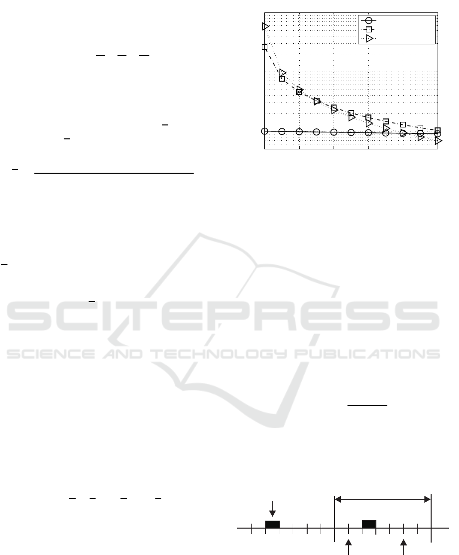
adaptation. Finally, Fig. 8 shows the approximated
gap distributions as a function of the interval length k
at a buyer concentration of (1− α) = 0, 2 and a buyer
probability of p
e
= 10
−2
.
Table 3: Estimation errors when using the Weibull distribu-
tion instead of the Wilhelm distribution.
(1−α) β
w
α
w
Error
0,0 0,010 1,000 0,000
0,1 0,013 0,460 0,007
0.2 0,033 0,310 0.002
0,3 0,119 0,264 0,007
0 20 40 60 80 100
0
0.2
0.4
0.6
0.8
1
interval length k →
u(k) →
Wilhelm
Exponential
Weibull
Figure 8: Approximated gap distributions as a function of
the interval length n at a buyer concentration of (1− α) =
0,2 and a buyer probability of p
e
= 10
−2
.
5 AGENT-BASED SIMULATION
In this section a model validation is carried out by
demonstrating that the model is a reasonable repre-
sentation of the investigated system (Martis, 2006).
Therefore, the objective of this section is compare
the probability P(n,e) with simulation outcomes ob-
tained by agent-based approach (Sajjad et al., 2016).
By agents relatively autonomous computational ob-
jects are understood. Agents of the same environment
Gap Distributions for Analysing Buyer Behaviour in Agent-based Simulation
27

Table 4: Comparison of the frequency γ
e
with the probability P(n,e) for memoryless buying scenarios.
block length number m
e
of probability mumber m of blocks in probability relative frequency
(theory) (simulation)
n of buying events p
e
simulated sample P(n,e) γ
e
5 2 0.01 200 0.001 0.000
5 1 0.01 200 0.048 0.040
5 2 0.1 200 0.073 0.051
5 1 0.1 200 0.328 0.328
7 4 0.1 142 0.003 0.007
7 2 0.1 142 0.128 0.078
5 2 0.5 200 0.031 0.030
5 1 0.5 200 0.156 0.197
7 4 0.5 142 0.273 0.234
7 2 0.5 142 0.164 0.170
may slightly differ in values of their properties, called
also attributes. Agents from different environments
may differ essentially. They exchange messages and
carry out activities influencing other agents and their
environment. Finally, agent activities are defined by
their own rules. Results of agent activities may be
message sending to other agents or the change of its
own state. The state of the agent may be changed
by other agents as well. Therefore according to vari-
ous authors, agents may have the following properties
(Ahrens et al., 2019):
• Intelligence: this property is implemented with
simple If then rules, fuzzy logic methods, built-in
neural networks, genetic algorithms, etc.
• Autonomy: agents are able to make decisions in-
dependently.
• Reactivity: agents have an ability to respond to
the activities of other agents and environment.
• Pro-activity: the agent may have a goal and are
programmed to reach it; the agent also may be
able to foresee possible negative events and to try
to avoid them.
• Adaptivity: agents may change their own rules of
behaviour responding to activities of other agents
and changes of environment as well as evaluating
accumulated statistics.
• Robustness: the ability to carry out activities and
survive in different environments.
• Goal-orientation: agents act according to their
goals and do nothing more.
• Mobility: agents may change their virtual place in
2D and 3D environments and they may be placed
on GIS map.
The process of making decisions when buyers enter
the shop was modelled using agent-based approach.
Each visitor was simulated as an autonomous agent
(Fig. 9). The visitors’ decisions were implemented as
rules. Each agent after entering the shop generated
a random decision to buy a product or service with
a given probability p
e
. Various statistics and logs of
the whole process were collected as well as various
properties of the burstiness were calculated (Ahrens
et al., 2019).
For the purposes of this work, the simulation was
supplemented for the memoryless buyer scenario by
the export of the sequence of one thousand agents’
decisions to the Excel file. Fig. 9 shows the structure
of an individual agent simulating the decision of an
individual buyer.
entering
exiting
buying
yes
no
deciding
Figure 9: Individual Agent simulating the decision of an
individual buyer.
These decisions known as binary customer be-
haviour were coded by series of 1 (decision to buy)
and 0 (not to buy). The series were splitted into m
blocks each of the length n (number of visitors, pat-
SENSORNETS 2019 - 8th International Conference on Sensor Networks
28

tern length). Therefore the total number of visitors is
given by n · m. For instance, when a pattern length
of n = 10 is considered, the series contained m = 100
blocks and therefore a series of n · m = 1000 visitors
is considered. Then the number m
e
of blocks con-
taining e buying events were counted. According to
the statistical definition of the probability, the relative
frequency
γ
e
=
m
e
m
(36)
is an estimation of the theoretical probability P(n,e).
Tab. 4 presents the comparison of the simulated rel-
ative frequency γ
e
with the probability P(n,e). As
Tab. 4 shows, the difference between the probability
P(n,e) and the relative frequency γ
e
is not large, and
can be be explained by the randomness of the agents’
behaviour. The match testifies the consistency of an-
alytical and simulation models.
6 CONCLUSIONS
The present research has successfully demonstrated
the adaptation of gap distribution functions from data
transmission theory in telecommunications to busi-
ness processes. The similar nature, namely bursty na-
ture, of bit-errors in telecommunications and buyers
in business management has been outlined. Conse-
quently, the present paper has emphasized the bursty
nature of business processes such as buying and sell-
ing, too. The complex process of buying by analysing
such properties of buyers’ behaviour as buyer proba-
bility and buyer concentration has been highlighted.
The research has resulted in proposing the use of
gaps for the description of the buying process. The
mathematical description of gap processes built on
the independence of gap intervals has been revealed
in the present paper. As shown by our research re-
sults, distribution functions with two parameters such
as Weibull or Wilhelm have been found to be an ade-
quate tool for the analysis of both, namely the buyers’
behaviour and the process of buying.
REFERENCES
Ahrens, A. (2000). A new digital channel model suitable
for the simulation and evaluation of channel error ef-
fects. In Colloquium on Speech Coding Algorithms
for Radio Channels, London (UK).
Ahrens, A., Purvinis, O., Zaˇsˇcerinska, J., and Andreeva, N.
(2015). Gap Processes for Modelling Binary Cus-
tomer Behavior. In 8th International Conference on
Engineering and Business Education, pages 8–13, Os-
tfold University College, Fredrikstad (Norway).
Ahrens, A., Purvinis, O., Zaˇsˇcerinska, J., Miceviˇciene, D.,
and Tautkus, A. (2019). Burstiness Management for
Smart, Sustainable and Inclusive Growth: Emerging
Research and Opportunities. IGI Global, 1 edition.
Ahrens, A. and Zaˇsˇcerinska, J. (2016). Gap Processes for
Analysing Buyers’ Burstiness in E-Business Process.
In International Conference on e-Business (ICE-B),
pages 8–13, Lisbon (Portugal).
Albanese, P. (2006). Inside Economic Man: Behavioral
Economics and Consumer Behavior. . In Altman, M.,
editor, Handbook of Contemporary Behavioral Eco-
nomics, volume 1, chapter 1, pages 3–77. Sharpe, 1
edition.
Axelrod, R. (2006). Agent-based Modeling as a Bridge Be-
tween Disciplines. In Tesfatsion, L. and Judd, K. L.,
editors, Handbook of Computational Economics, vol-
ume 2, chapter 33, pages 1565–1584. Elsevier, 1 edi-
tion.
Elliott, E. O. (1963). Estimates of Error Rates for Codes on
Burst-Noise Channels. Bell System Technical Journal,
42(5):1977–1997.
Gilbert, E. N. (1960). Capacity of a Burst-Noise Channel.
Bell System Technical Journal, 39:1253–1265.
Martis, M. S. (2006). Validation of Simulation Based Mod-
els: A Theoretical Outlook. Electronic Journal of
Business Research Methods, 4(1):39–46.
Sajjad, M., Singh, K., Paik, E., and Ahn, C. (2016). So-
cial Simulation: The need of data-driven agent-based
modelling Approach. In 2016 18th International
Conference on Advanced Communication Technology
(ICACT), pages 818–821.
Tesfatsion, L. (2006). Agent-Based Computational Eco-
nomics: A Constructive Approach to Economic The-
ory. In Tesfatsion, L. and Judd, K. L., editors, Hand-
book of Computational Economics, volume 2, pages
831–880. Elsevier, 1 edition.
Wilhelm, H. (1976). Daten¨ubertragung (in German).
Milit¨arverlag, Berlin.
Gap Distributions for Analysing Buyer Behaviour in Agent-based Simulation
29