Boosting 3D Shape Classification with Global Verification and
Redundancy-free Codebooks
Viktor Seib, Nick Theisen and Dietrich Paulus
Active Vision Group (AGAS), University of Koblenz-Landau, Universit
¨
atsstr. 1, 56070 Koblenz, Germany
http://agas.uni-koblenz.de
Keywords:
Shape Classification, Global Verification, Mobile Robotics, Implicit Shape Models, Point Clouds, Codebooks.
Abstract:
We present a competitive approach for 3D data classification that is related to Implicit Shape Models and
Naive-Bayes Nearest Neighbor algorithms. Based on this approach we investigate methods to reduce the
amount of data stored in the extracted codebook with the goal to eliminate redundant and ambiguous feature
descriptors. The codebook is significantly reduced in size and is combined with a novel global verification
approach. We evaluate our algorithms on typical 3D data benchmarks and achieve competitive results despite
the reduced codebook. The presented algorithm can be run efficiently on a mobile computer making it suitable
for mobile robotics applications. The source code of the developed methods is made publicly available to
contribute to point cloud processing, the Point Cloud Library (PCL) and 3D classification software in general.
1 INTRODUCTION
Current research for object classification and de-
tection focuses on deep neural networks for 2D image
data (Lin et al., 2017), (He et al., 2017). However,
affordable 3D sensors increase the demand for 3D
data processing. Consequently, approaches exploiting
depth data from RGBD-cameras have been proposed
(Eitel et al., 2015), (Zia et al., 2017). Neural networks
using volumetric (Maturana and Scherer, 2015), (Wu
et al., 2015), (Garcia-Garcia et al., 2016) or point
cloud data (Qi et al., 2017) for object classification
are still rare. PointNet
1
(Qi et al., 2017) is currently
one of the best approaches in that area.
Our research is well informed about the advan-
ces achieved in the field of convolutional neural net-
works for object classification. In this work we ad-
here to a classic approach without the application of
neural networks. This has certain benefits. The trai-
ning phase takes significantly less time and computa-
tional resources. Further, the selection of parameters
for training is straight forward and does not require
time consuming tuning in a trial-and-error fashion.
Finally, the trained model runs efficiently on a mo-
bile computer which makes it well-suited for mobile
robotics applications. One downside, is that neural
1
The algorithms presented in (Garcia-Garcia et al.,
2016) and (Qi et al., 2017) are both dubbed “PointNet”.
networks allow to use more training data without in-
creasing the model size. Among others, this shortco-
ming of codebook-based approaches is addressed in
this work.
The Point Cloud Library (PCL)
2
addresses the de-
mand for 3D data processing by providing a frame-
work with a standardized data format and many al-
gorithms. Further, the PCL offers a complete proces-
sing pipeline for 3D object recognition and provides
an adaption of the well-known Implicit Shape Model
(ISM) approach (Leibe et al., 2004) to 3D data. The
3D variant of ISM constructs a geometric alphabet of
shape appearances, the codebook, rather than a visual
alphabet of 2D image patches (Leibe et al., 2004).
We present several methods to estimate a descrip-
tor’s relevance during training to obtain a more des-
criptive codebook and omit redundancies. Our se-
cond contribution is a global verification approach
that boosts the classification performance. Finally, as
a third contribution, the source code of our contribu-
tions is made publicly available
3
. Our algorithm is
competitive with standard approaches for 3D object
classification on commonly used datasets. By provi-
ding the source code we hope to make a valuable con-
tribution to open-source 3D classification software.
2
Point Cloud Library: http://pointclouds.org/
3
Code, documentation and examples available at https:
//github.com/vseib/PointCloudDonkey
Seib, V., Theisen, N. and Paulus, D.
Boosting 3D Shape Classification with Global Verification and Redundancy-free Codebooks.
DOI: 10.5220/0007312402570264
In Proceedings of the 14th International Joint Conference on Computer Vision, Imaging and Computer Graphics Theory and Applications (VISIGRAPP 2019), pages 257-264
ISBN: 978-989-758-354-4
Copyright
c
 2019 by SCITEPRESS – Science and Technology Publications, Lda. All rights reserved
257

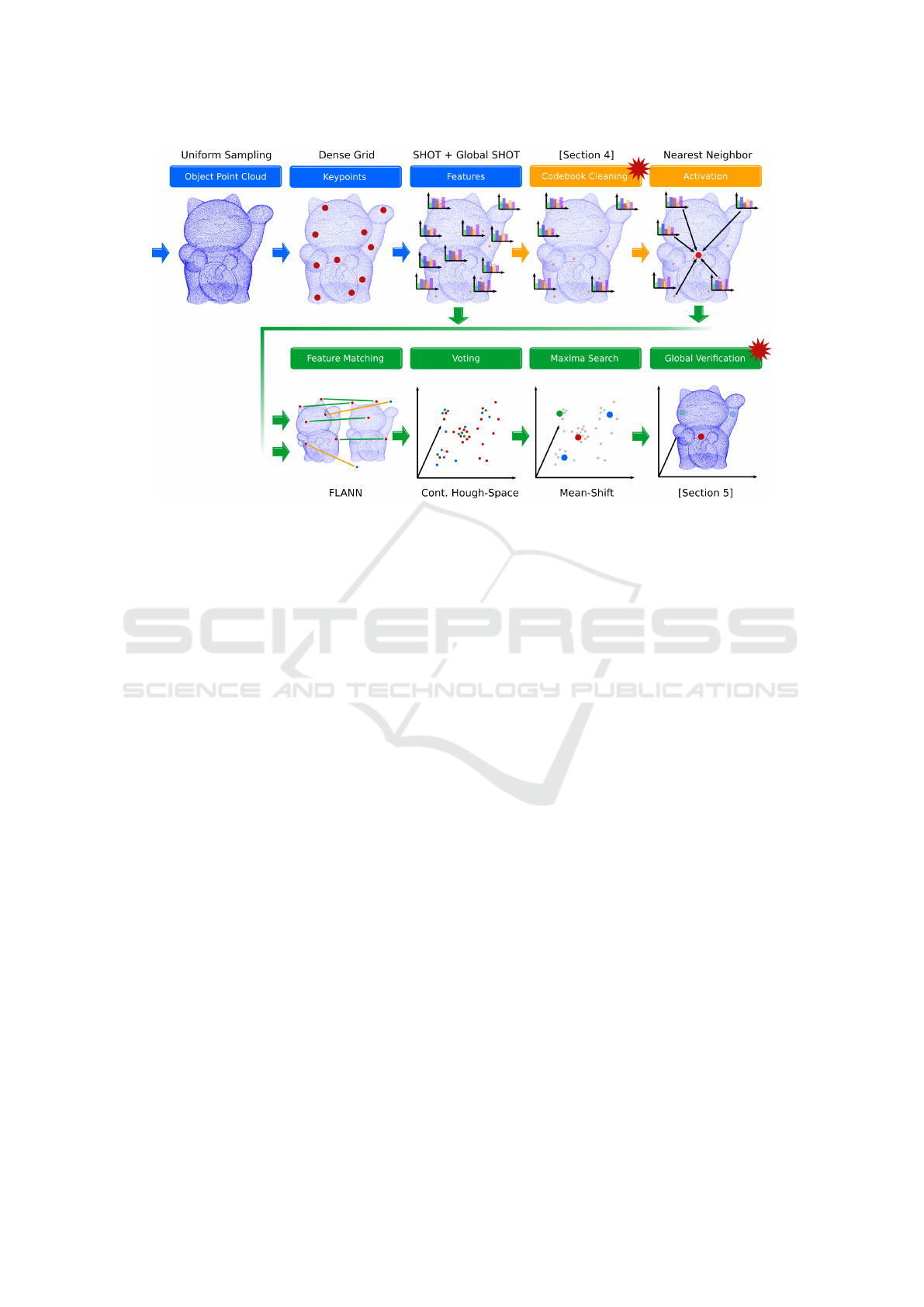
Figure 1: The pipeline used in this work. Blue steps are common for both, training (orange) and classification (green). The
contributions of this work are marked with a red star. The maneki-neko (lucky cat) model is intellectual property of user bs3
(downloaded from https://www.thingiverse.com/thing:923097).
Section 2 presents related work on codebook re-
duction. Our point cloud processing pipeline is pre-
sented in Section 3 with the contributions for co-
debook cleaning (Section 4) and global verification
(Section 5). Section 6 presents and discusses an ex-
tensive evaluation of the proposed algorithms, while
Section 7 concludes the paper.
2 RELATED WORK
A common technique to reduce the size of the co-
debook is vector quantization. However, this is also
one of the main reasons for the inferior performance
of Nearest-Neighbor-based methods (Boiman et al.,
2008). Consequently, feature clustering is omitted by
approaches using 3D data (Salti et al., 2010), (Tom-
bari and Di Stefano, 2010) and some Naive-Bayes Ne-
arest Neighbor methods (McCann and Lowe, 2012).
The ISM algorithm contained in the PCL (Knopp
et al., 2010) also uses vector quantization to reduce
the codebook size. Other approaches argue against
verctor quantization (Salti et al., 2010), (Tombari and
Di Stefano, 2010), (Seib et al., 2015). The latter rea-
dapts the continuous hough-space of the original ISM
algorithm to 3D data in contrast to the discrete voting
spaces of other ISM adaptations.
Other ways of handling ambiguous features is an
optimization step during training that assigns weig-
hts to individual features (Liu et al., 2015), (McCann
and Lowe, 2012). These approaches improve classi-
fier performance in their respective domains. Howe-
ver, they do not aim at cleaning out feature descriptors
to reduce the codebook size.
Due to the limitations of clustered codebooks a
random feature selection was proposed (Cui et al.,
2015). Surprisingly, in some cases a randomly redu-
ced codebook performs even better than the complete
codebook. These experiments show that some of the
features are less descriptive than others. We are thus
interested in finding an approach that can judge the fe-
atures and maintain only the strong descriptors, while
the weak or ambiguous ones are discarded.
Alternatively, the size of the codebook can be re-
duced by reducing the entry size instead of reducing
the number of entries. Recently, (Prakhya et al., 2015)
proposed to convert SHOT into a binary descriptor,
B-SHOT, to reduce its memory requirements. Furt-
her, recent advances in deep learning allow to le-
arn compact feature descriptors for 3D data (Khoury
et al., 2017), (Schmidt et al., 2017). In (Khoury et al.,
2017) Compact Geometric Features (CGF) are propo-
sed that outperform hand-crafted features (including
SHOT) in scan registration. Taking these recent rese-
arch into account we will compare our contributions
with the B-SHOT and CGF descriptors.
3 PIPELINE DESCRIPTION
For our own approach we re-implement the complete
ISM pipeline (Figure 1) using the PCL. We take inspi-
VISAPP 2019 - 14th International Conference on Computer Vision Theory and Applications
258

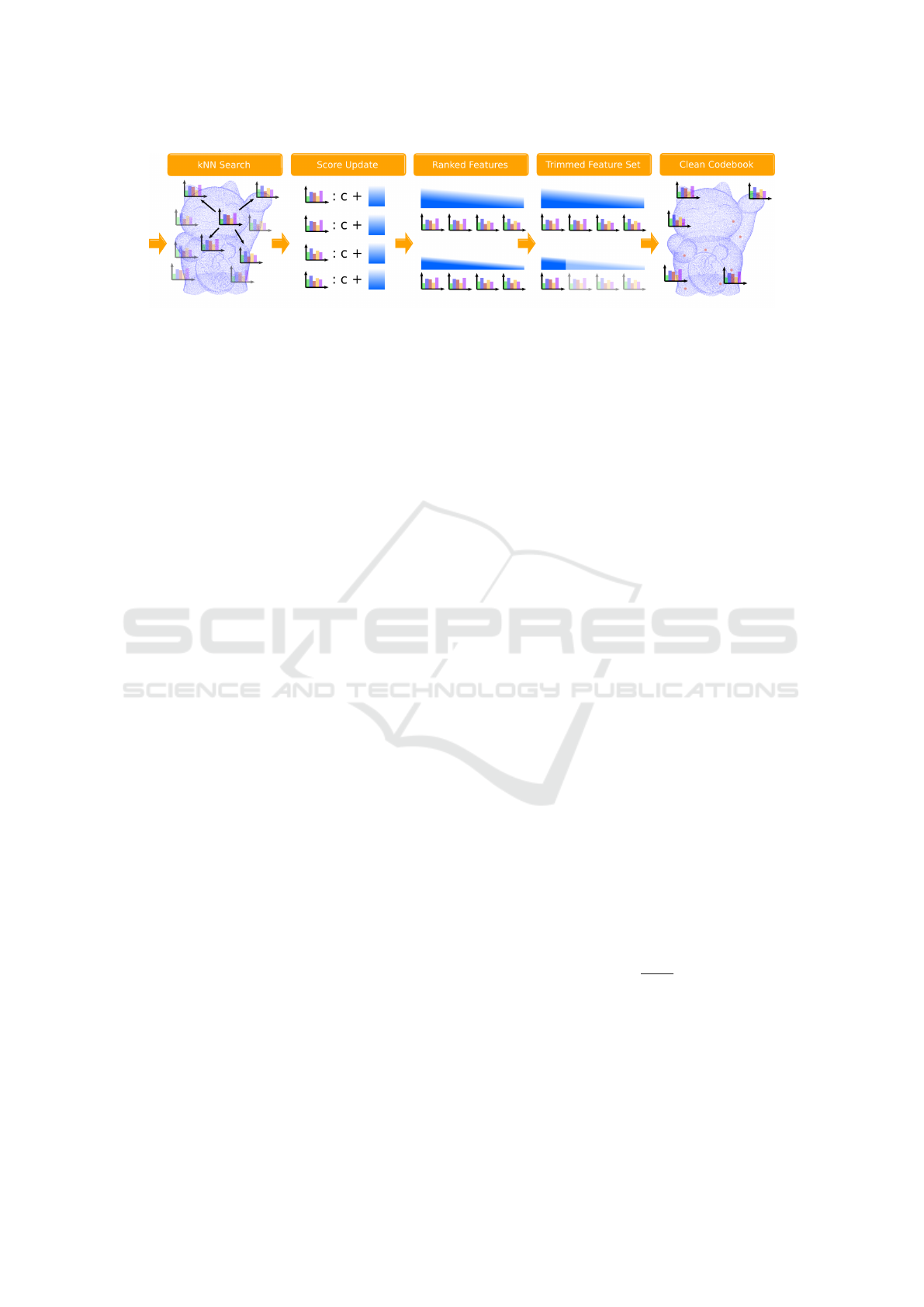
Figure 2: All features serve as input to the codebook cleaning pipeline. A set of nearest neighbors is found for each feature
and their scores are updated (see text). All features are ranked and trimmed based on their score to obtain a clean codebook.
ration from Naive-Bayes Nearest Neighbor (NBNN)
(McCann and Lowe, 2012), (Boiman et al., 2008) and
combine it with the localized hough-voting scheme
of ISM (Seib et al., 2015), (Tombari and Di Ste-
fano, 2010). The design choices we make for each
of the pipeline steps are shown in Figure 1. We ex-
tract keypoints on a dense grid and compute SHOT
descriptors for the keypoint locations. From all des-
criptors of the PCL, SHOT performed best in terms of
accuracy and speed in our experiments. In the training
pipeline (orange) we omit clustering and retain all fe-
atures. The resulting codebook is formed by a strict k-
NN activation with k = 1, i.e. every feature only votes
for itself. In the classification pipeline (green) we ef-
ficiently match descriptors using FLANN and choose
a continuous voting space. Finally, a mean-shift max-
ima search yields object hypotheses. The described
pipeline (without the steps marked with red stars in
Figure 1) serves as a baseline for the evaluation of the
contributions proposed here.
4 CODEBOOK CLEANING
We present two algorithms to judge the relevance of a
feature in this section. The two presented algorithms
share a common idea: they compute a score for each
feature and rank the features according to that score.
The score updates are applied to the k nearest neig-
hbors of a query feature
~
f
q
instead of the feature itself.
Therefore, the resulting score value c of each feature
~
f is a sum of individual update values
c =
m
∑
i
v
i
. (1)
The number of update values m varies from feature to
feature as it indicates how often feature
~
f was within
the k nearest neighbors of all query features. Finally,
a fixed ratio of features will be selected from the ran-
ked list. The process of codebook cleaning is applied
during training and is shown in Figure 2.
4.1 Incremental Ranking
McCann and Lowe (McCann and Lowe, 2012) pro-
pose a classification rule that updates the posterior
probability of a class by an increment derived from
the k nearest neighbors of a query feature
~
f
q
. For
the purpose of codebook cleaning we take inspiration
from McCann and Lowe and define the Incremental
ranking, with the score c
inc
. The idea is to derive a fe-
ature increment instead of a class increment that com-
pares a feature’s distance with a background distance.
Our experiments have shown that an individual back-
ground distance d
b
per feature yields best results and
is less dependent on the choice of k.
Given a query feature
~
f
q
and its k +1 nearest neig-
hbors
~
f
j
, j ∈ {1,...,k,k + 1} we update the coeffi-
cients of the first k neighbors by
v
j
= d
j
− d
b
= k
~
f
q
−
~
f
j
k
2
− k
~
f
q
−
~
f
j+1
k
2
. (2)
4.2 KNN-Activation Ranking
The KNN-Activation ranking simulates the classifi-
cation process during training. The updates v
i
for the
corresponding score c
ka
are defined in various ways.
We define a base update value u = 1. In the simplest
case we update the score of the k nearest neighbors
~
f
j
, j ∈ {1, . . .,k} of a query feature
~
f
q
by
v
j
= u . (3)
The second score increment uses the descriptor dis-
tance d = k
~
f
q
−
~
f
j
k
2
between the query feature
~
f
q
and
its j-th neighbor
~
f
j
and is defined as
v
j
=
u
d + 1
. (4)
Thereby, the similarity of the features is considered in
the update. The update becomes bigger with an in-
creasing descriptor similarity (favoring similar featu-
res). Another possibility is to make the updates smal-
ler with an increasing descriptor similarity (favoring
unique features):
v
j
= u · exp(d) . (5)
Boosting 3D Shape Classification with Global Verification and Redundancy-free Codebooks
259

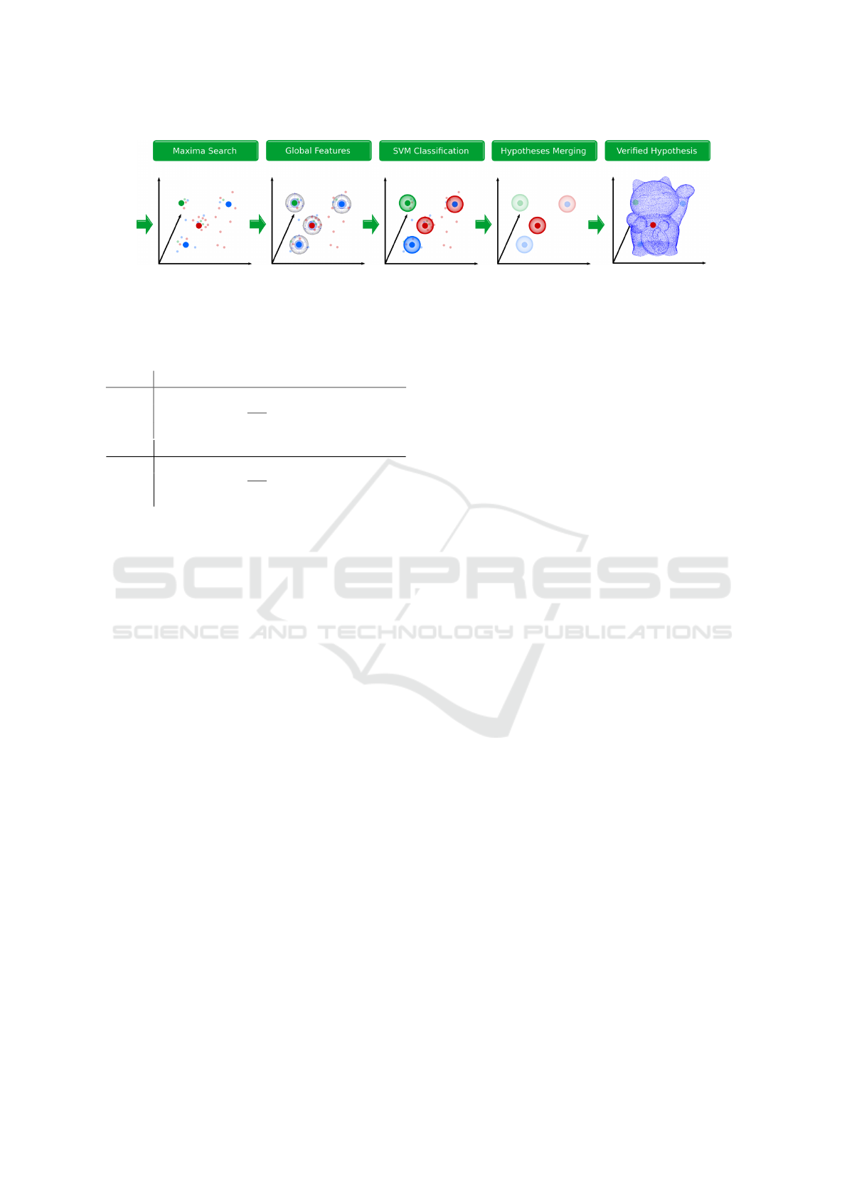
Figure 3: The global verification step takes the maxima found by the local classifier as input. A global feature is computed
for the maxima locations. The global features are classified and merged to form the final object hypothesis.
Table 1: Assignment of indexed names to the investiga-
ted variants of the KNN-Activation Coefficient c
ka
from
Section 4.2.
name without keypoint position (u = 1)
c
ka1
1 Eq. 3
c
ka2
1
d+1
Eq. 4
c
ka3
1 · exp(d) Eq. 5
name with keypoint pos. (u from Eq. 6)
c
ka4
u Eq. 3
c
ka5
u
d+1
Eq. 4
c
ka6
u · exp(d) Eq. 5
So far, only the descriptor distance d (feature si-
milarity) was taken into account. We further redefine
the base update value u = 1 as
u = exp(|c
j
− c
q
|) (6)
for all of the above equations. The center distances c
j
and c
q
denote the distance of a keypoint of a feature
~
f
j
and
~
f
q
to the object’s centroid. Thereby, also the
relative position of a feature’s keypoint is considered
in the score increment. To be able to easily refer to
the different variants of the c
ka
scores defined here we
summarize them in Table 1 and assign indexed names.
5 GLOBAL VERIFICATION
While local features provide good robustness against
noise and clutter they still produce wrong maxima.
This effect is handled by including a verification step
into the object recognition pipelines (Aldoma et al.,
2012), (Maji and Malik, 2009).
We propose a different verification strategy,
shown in Figure 3. Our hypothesis verification is ba-
sed on a classifier that takes global features as input
(in the following named global classifier, as apposed
to the local classifier based on SHOT features). The
global classifier computes an object hypothesis inde-
pendently from the hypotheses of the local classifier.
In a second step, all local and global hypotheses are
fused. The motivation behind this approach is to eli-
minate wrong maxima and strengthen maxima where
the global classifier supports the classification hypot-
hesis.
We distinguish two use cases for our global veri-
fication approach. In the first use case the input data
contains a single object (e.g. a previously segmen-
ted object with known location, but unknown class
label). In this case a global feature descriptor is com-
puted on the input. This (single) result is merged with
all hypotheses from the local classifier. In the second
use case the input data contains an unknown number
of objects and possibly some clutter. The locations
of the maxim are used to extract a partial point cloud
for each maximum and compute a global feature des-
criptor. Each of the classification results of the global
classifier is merged with the corresponding maximum
from the local classifier to obtain the final object label.
Despite the global feature descriptors in the PCL
our own experiments have shown a better perfor-
mance when using an adaption of SHOT to a glo-
bal scale. We train a two-class SVM in a “one-vs.-
all”-fashion for each of the classes with the global
descriptors. The classification output is a class label
and score s ∈ [0,1] representing the probability for the
found label.
The maxima from the local classifier and the cor-
responding classification results from the global clas-
sifier are merged to obtain the final classification re-
sult and weight. The merging is based on the local
and global labels l
l
,l
g
∈ N, as well as on the local and
global weight w
l
,w
g
∈ R of each maximum. Additio-
nally, the highest local weight ˆw
l
∈ R is used when
classifying isolated objects. The merging function
f
m
: N
2
× R
3
→ N × R that takes both labels, both
weights and the overall highest local weight as inputs
and outputs the final classification label and weight.
We test multiple definitions of this function f
m
in
our evaluation. In the first use case the global clas-
sification result is the same for all maxima obtained
from the local classifier. We search for the global la-
bel among the top-ranked maxima from the local clas-
sifier. If the global label is among the top results and
VISAPP 2019 - 14th International Conference on Computer Vision Theory and Applications
260

Figure 4: Example objects contained in the datasets used
for evaluation.
has a high weight, it is considered the true label:
f
m1
(·) =
(
l
g
, ˆw
l
+ ε if w
l
> t
r
· ˆw
l
∧ l
g
= l
l
l
l
,w
l
otherwise.
(7)
In this case t
r
∈ [0, 1] is the rate threshold determining
which local maxima are considered to be top results.
The function f
m1
upweights a maximum by adding a
small increment ε to the highest available weight.
In the general case of an unknown number of ob-
jects in the input data, the preferred solution is to
merge the classification results of the local and the
global classifier per maximum. An individual global
classification is carried out for each of the maxima
from the local classifier. The corresponding maxima
will be upvoted using f
m2
:
f
m2
(·) =
(
l
g
,w
l
· c
f
if l
g
= l
l
l
l
,w
l
otherwise.
(8)
Function f
m2
uses a fixed constant factor c
f
> 1 to
emphasize maxima where both classifiers agree on a
label. Further, we evaluate the merging function f
m3
,
which is similar to f
m2
, but is parameter free:
f
m3
(·) =
(
l
g
,w
l
· (1 + w
g
) if l
g
= l
l
l
l
,w
l
otherwise.
(9)
If both classifiers agree on the label, the resulting
weight is determined based on the global weight. By
adding the constant 1 we ensure to never downweight
a maximum from the local classifier.
6 EVALUATION AND RESULTS
We evaluate our approach on datasets used to bench-
mark 3D classification and shape retrieval algorithms.
We convert the object meshes of these datasets to
point clouds and scale each model to the unit circle
for classification. Example objects are shown in Fi-
gure 4.
Aim@Shape-Watertight (ASW) (Giorgi et al.,
2007) 20 object classes, 200 object for training
and for testing.
McGill Dataset (MCG)
4
19 classes with articulated
objects, 234 for training and 223 for testing.
4
McGill: www.cim.mcgill.ca/~shape/benchMark/
Princeton Shape Benchmark (PSB)
5
7 classes with
907 objects for training and for testing.
Shrec-12 (SH12)
6
shape retrieval benchmark 60
classes, 600 objects for training and for testing.
ModelNet (MN40 and MN10) (Wu et al., 2015):
Full dataset (MN40, 40 classes) and its subset
(MN10, 10 classes) used to benchmark neural net-
works for shape classification. MN40: 9843 ob-
jects for training, 2468 for testing. MN10: 3991
objects for training and 908 for testing. We use
only a subset of the training data. Contrary to ot-
her datasets, the standard metric for these two da-
tasets is average per class accuracy and will be
reported accordingly in all tables.
We first compare our algorithm to other approa-
ches to establish a baseline for further evaluations.
In particular, we compare our work to (McCann and
Lowe, 2012) and (Seib et al., 2015) because of its si-
milarity to the default pipeline and to (Knopp et al.,
2010) as it is the ISM implementation in the PCL. Ad-
ditionally, we compare with the approach of Ganihar
et al.(Ganihar et al., 2014), the descriptor B-SHOT
(Prakhya et al., 2015) and the deep learned feature
CGF (Khoury et al., 2017). In the latter two cases we
use the code provided by the authors of the approa-
ches. The authors of CGF provide different trained
models on two distinct datasets. We report results for
the best performing of these models in our pipeline
(CGF descriptor with 40 dimensions trained on laser
scan data). Finally, we compare our algorithm with
recent neural networks for shape classification on the
ModelNet dataset.
The baseline comparison with non deep learning
approaches is presented in Table 2. The classifica-
tion results reported for (McCann and Lowe, 2012)
are based on our own implementation. Our base pi-
peline performs best on two datasets. We observe that
the SHOT descriptor is a good choice since it outper-
forms the B-SHOT and CGF descriptors in the base
pipeline. CGF performs well for scan registration as
reported in (Khoury et al., 2017), however, it is not
descriptive enough for shape classification.
6.1 Reduction of Codebook Size
The following evaluation is carried out with the two
datasets ASW (rigid shapes) and MCG (articulated
shapes) to find best hyperparameters. Our propo-
sed codebook size reduction methods are additio-
nally compared to a random codebook generation
5
PSB: shape.cs.princeton.edu/benchmark/
6
Shrec-12: www.itl.nist.gov/iad/vug/sharp/contest/
2012/Generic3D/
Boosting 3D Shape Classification with Global Verification and Redundancy-free Codebooks
261

Table 2: Comparison of our baseline results with approaches in literature. We report the overall accuracy for ASW, MCG,
PSB and SH12 and the average per class accuracy for MN10 and MN40. Best result per dataset is shown in bold.
Dataset McCann and Lowe Seib et al. Knopp et al. (PCL) Ganihar et al.
(McCann and Lowe, 2012) (Seib et al., 2015) (Knopp et al., 2010) (Ganihar et al., 2014)
ASW 87.0 85.0 - -
MCG 82.5 - - -
PSB 66.6 61.6 58.3 67.9
SH12 73.2 - - 66.4
Dataset this work (base pipeline) with different feature descriptors
CGF (Khoury et al., 2017) B-SHOT (Prakhya et al., 2015) SHOT (Tombari et al., 2010)
ASW 80.5 87.0 90.0
MCG 73.1 78.9 85.2
PSB 58.7 62.0 67.0
SH12 58.3 64.3 70.2
MN10 - - 62.4
MN40 - - 71.9
Table 3: Comparison of the proposed ranking methods for
codebook cleaning and the baseline. The results obtained
refer to a codebook size of 75% compared to the baseline.
Coefficient ASW MCG
own baseline 90 85.2
c
inc
89 83.9
c
ka2
91 84.3
c
ka4
89 83.0
random average 88.9 83.7
Table 4: Comparison of merging functions for global veri-
fication. Values in brackets indicate the applied parameter
values. All results are better than the baseline.
Merging function ASW MCG
f
m1
(0.7) 91.5 86.6
f
m2
(2.0) 92 86.6
f
m3
(-) 91 86.6
(Cui et al., 2015). We randomly select 75% of all
features to compare with our codebook cleaning met-
hod. The random selection was run 100 times and the
average results are reported.
Table 3 reports the results on codebook cleaning
using the proposed ranking methods (for clarity, we
only report the best and the worst result for c
ka
). The
results were obtained by taking the best 75% of featu-
res according to their computed ranking. A codebook
reduced with our approach hardly looses descriptive-
ness and the results almost stay the same as the base-
line. The loss for the MCG dataset is slightly higher,
since this dataset contains articulated objects.
6.2 Global Verification
We have introduced three hypothesis merging functi-
ons for the purpose of global verification. Two of
Table 5: Combination of global verification and codebook
cleaning (reduction to 75%). Bold typeset indicates results
that are equal or better than our baseline.
Dataset c
ka3
+ f
m2
(2.0) c
ka5
+ f
m2
(2.0)
ASW 93.0 93.0
MCG 86.1 84.3
PSB 67.8 67.1
SH12 71.7 73.8
MN10 - 83.8
MN40 - 75.4
these functions depend on a parameter, while the third
is a parameter-free approach. However, our experi-
ments have shown that the choice of the parameter (in
a reasonable range) hardly effects the classification
results. The results of the global classifier combined
with the base pipeline (without codebook reduction)
are reported in Table 4. Adding global features and
the proposed merging functions to the baseline classi-
fier improves the classification by about 2% for ASW
(92%) and about 1% for the MCG (86%) dataset. The
choice of the merging function (and its parameters)
has only little influence on the result.
6.3 Combining Codebook Reduction
and Global Verification
In this evaluation we test all datasets and reduce their
codebooks to 75%. For clarity, we can not report re-
sults for all ranking and merging functions. However,
we observe that the ranking not using the descriptor
similarity (c
ka1
and c
ka4
, Equation 3) perform worse
throughout all experiments. Whether the keypoint po-
sition (Equation 6) is used or not has a less significant
impact. The two ranking methods favoring similar fe-
VISAPP 2019 - 14th International Conference on Computer Vision Theory and Applications
262

Table 7: Comparison of the final evaluation results. The proposed contributions overcome the baseline on all datasets despite
the reduction of the codebook data. Bold typeset indicates results better than state of the art and the baseline. We report the
overall accuracy for ASW, MCG, PSB and SH12 and the average per class accuracy for MN10 and MN40.
best results in this work this work (contributions)
Dataset related work (own baseline) codebook size
100% 75% 50% 25%
ASW 87.0 (McCann and Lowe, 2012) 90.0 92.0 93.0 93.5 92.0
MCG 82.5 (McCann and Lowe, 2012) 85.2 86.6 86.1 85.6 83.0
PSB 67.9 (Ganihar et al., 2014) 67.0 68.4 67.8 67.9 65.3
SH12 73.2 (McCann and Lowe, 2012) 70.2 74.5 73.8 70.8 65.5
MN10 92.0 (Maturana and Scherer, 2015) 62.4 67.3 83.8 83.1 81.4
MN40 86.2 (Qi et al., 2017) 71.9 76.2 75.4 74.4 72.5
Table 6: Comparison of our proposed contributions with
deep learning approaches on the MN10 and MN40 datasets.
MN10 MN40
this work (codebook size 75% 83.8 75.4
+ global verification)
PointNet 76.7 -
(Garcia-Garcia et al., 2016)
ShapeNets (Wu et al., 2015) 83.5 77.3
VoxNet 92.0 83.0
(Maturana and Scherer, 2015)
PointNet (Qi et al., 2017) - 86.2
atures (c
ka2
and c
ka5
, Equation 4) are better for small
codebook reductions. On the other hand, if the co-
debook is reduced by a great extent, ranking methods
favoring unique features (c
ka3
and c
ka6
, Equation 5)
perform best. For a better overview we only show
the results of two coefficients, both combined with the
merging function f
m2
(Equation 8) in Table 5. We ob-
serve that the combination of our proposed codebook
cleaning technique combined with the global verifica-
tion approach retains a high descriptiveness and over-
all good classification results. In fact, the codebooks
with 75% of all features still performs better then the
established baseline in almost all cases.
Table 6 compares our proposed pipeline with re-
cent deep learning approaches on the MN10 and
MN40 datasets. Note that our pipeline surpasses two
of the deep learning approaches on the MN10 dataset.
However, is is also far behind the leading approaches
VoxNet (Maturana and Scherer, 2015) and PointNet
(Qi et al., 2017).
Finally, Table 7 summarizes all evaluation results.
Our contributions overcome the state of the art on
classic (non deep learning) approaches on the four
smaller datasets. This holds for most cases, even if
the size of the codebook is significantly reduced. This
supports our hypothesis that our codebook cleaning
successfully eliminates less descriptive and ambigu-
ous features. The more recent datasets MN10 and
MN40 are usually applied to benchmark deep lear-
ning shape classification approaches. Although our
contributions significantly improve over the baseline,
some deep learning approaches are still better. Howe-
ver, Table 6 shows that our classic approach is com-
petitive with some of the deep learning pipelines.
The average classification times per object for
our baseline method were measured on a six years
old notebook with an Intel Core i7-2760QM CPU @
2.40GHz and are on average around 0.4 s for the ASW
and MCG datasets, around 1 s for the PSB and the
SH12 datasets and around 2 to 5 s on the large MN40
dataset (depending on codebook size). The classifi-
cation times increase by about 0.2 s due to the SVM
classification if the described contributions are app-
lied additionally. We therefore consider our approach
suitable for mobile robotics applications.
7 CONCLUSION
The combination of the presented algorithms allows
to significantly reduce the amount of data used for
codebook construction. The merging functions for
global features mostly provide stable results, even if
the parameters are varied. Despite the reduced co-
debook size, the classification performance is impro-
ved for all datasets compared to the baseline (Table 7)
and overcomes the state of the art of classic appro-
aches and is competitive with some deep learning
methods. The proposed codebook reduction method
is computed during training and is computationally
light-weight. We consider our methods and the pro-
vided open-source software as a valuable contribution
to the 3D vision community. In future work we will
investigate methods to bridge the gap between classic
and deep learning approaches.
Boosting 3D Shape Classification with Global Verification and Redundancy-free Codebooks
263

REFERENCES
Aldoma, A., Marton, Z.-C., Tombari, F., Wohlkinger, W.,
Potthast, C., Zeisl, B., Rusu, R. B., Gedikli, S., and
Vincze, M. (2012). Tutorial: Point cloud library:
Three-dimensional object recognition and 6 dof pose
estimation. IEEE Robotics & Automation Magazine,
19(3):80–91.
Boiman, O., Shechtman, E., and Irani, M. (2008). In de-
fense of nearest-neighbor based image classification.
In Computer Vision and Pattern Recognition, 2008.
CVPR 2008. IEEE Conf. on, pages 1–8. IEEE.
Cui, S., Schwarz, G., and Datcu, M. (2015). Image clas-
sification: No features, no clustering. In Image Pro-
cessing (ICIP), 2015 IEEE Int. Conf. on, pages 1960–
1964. IEEE.
Eitel, A., Springenberg, J. T., Spinello, L., Riedmiller, M.,
and Burgard, W. (2015). Multimodal deep learning
for robust rgb-d object recognition. In Intelligent Ro-
bots and Systems (IROS), 2015 IEEE/RSJ Int. Conf.
on, pages 681–687. IEEE.
Ganihar, S. A., Joshi, S., Setty, S., and Mudenagudi, U.
(2014). Metric tensor and christoffel symbols based
3d object categorization. In Asian Conf. on Computer
Vision, pages 138–151. Springer.
Garcia-Garcia, A., Gomez-Donoso, F., Garcia-Rodriguez,
J., Orts-Escolano, S., Cazorla, M., and Azorin-Lopez,
J. (2016). Pointnet: A 3d convolutional neural net-
work for real-time object class recognition. In Neural
Networks (IJCNN), 2016 International Joint Conf. on,
pages 1578–1584. IEEE.
Giorgi, D., Biasotti, S., and Paraboschi, L. (2007). Shape re-
trieval contest 2007: Watertight models track. SHREC
competition, 8(7).
He, K., Gkioxari, G., Doll
´
ar, P., and Girshick, R. (2017).
Mask r-cnn. In Computer Vision (ICCV), 2017 IEEE
Int. Conf. on, pages 2980–2988. IEEE.
Khoury, M., Zhou, Q.-Y., and Koltun, V. (2017). Le-
arning compact geometric features. arXiv preprint
arXiv:1709.05056.
Knopp, J., Prasad, M., Willems, G., Timofte, R., and
Van Gool, L. (2010). Hough transform and 3d surf
for robust three dimensional classification. In ECCV
(6), pages 589–602.
Leibe, B., Leonardis, A., and Schiele, B. (2004). Combined
object categorization and segmentation with an impli-
cit shape model. In ECCV’ 04 Workshop on Statistical
Learning in Computer Vision, pages 17–32.
Lin, T.-Y., Goyal, P., Girshick, R., He, K., and Dollar, P.
(2017). Focal loss for dense object detection. In 2017
IEEE Int. Conf. on Computer Vision (ICCV), pages
2999–3007. IEEE.
Liu, Q., Puthenputhussery, A., and Liu, C. (2015). Novel
general knn classifier and general nearest mean clas-
sifier for visual classification. In Image Processing
(ICIP), 2015 IEEE Int. Conf. on, pages 1810–1814.
IEEE.
Maji, S. and Malik, J. (2009). Object detection using a max-
margin hough transform. In Computer Vision and Pat-
tern Recognition, 2009. CVPR 2009. IEEE Conf. on,
pages 1038–1045. IEEE.
Maturana, D. and Scherer, S. (2015). Voxnet: A 3d convo-
lutional neural network for real-time object recogni-
tion. In Intelligent Robots and Systems (IROS), 2015
IEEE/RSJ Int. Conf. on, pages 922–928. IEEE.
McCann, S. and Lowe, D. G. (2012). Local naive bayes
nearest neighbor for image classification. In Computer
Vision and Pattern Recognition (CVPR), 2012 IEEE
Conf. on, pages 3650–3656. IEEE.
Prakhya, S. M., Liu, B., and Lin, W. (2015). B-shot: A
binary feature descriptor for fast and efficient keypoint
matching on 3d point clouds. In Intelligent Robots and
Systems (IROS), 2015 IEEE/RSJ Int. Conf. on, pages
1929–1934. IEEE.
Qi, C. R., Su, H., Mo, K., and Guibas, L. J. (2017). Point-
net: Deep learning on point sets for 3d classification
and segmentation. Proc. Computer Vision and Pattern
Recognition (CVPR), IEEE, 1(2):4.
Salti, S., Tombari, F., and Di Stefano, L. (2010). On the
use of implicit shape models for recognition of object
categories in 3d data. In ACCV (3), Lecture Notes in
Computer Science, pages 653–666.
Schmidt, T., Newcombe, R., and Fox, D. (2017). Self-
supervised visual descriptor learning for dense corre-
spondence. IEEE Robotics and Automation Letters,
2(2):420–427.
Seib, V., Link, N., and Paulus, D. (2015). Pose estimation
and shape retrieval with hough voting in a continuous
voting space. In German Conf. on Pattern Recogni-
tion, pages 458–469. Springer.
Tombari, F. and Di Stefano, L. (2010). Object recognition in
3d scenes with occlusions and clutter by hough voting.
In Image and Video Technology (PSIVT), 2010 Fourth
Pacific-Rim Symposium on, pages 349–355. IEEE.
Tombari, F., Salti, S., and Di Stefano, L. (2010). Unique
signatures of histograms for local surface description.
In Proc. of the European Conf. on computer vision
(ECCV), ECCV’10, pages 356–369. Springer-Verlag.
Wu, Z., Song, S., Khosla, A., Yu, F., Zhang, L., Tang, X.,
and Xiao, J. (2015). 3d shapenets: A deep represen-
tation for volumetric shapes. In Proceedings of the
IEEE conference on computer vision and pattern re-
cognition, pages 1912–1920.
Zia, S., Y
¨
uksel, B., Y
¨
uret, D., and Yemez, Y. (2017). Rgb-
d object recognition using deep convolutional neural
networks. In 2017 IEEE Int. Conf. on Computer Vision
Workshops (ICCVW), pages 887–894. IEEE.
VISAPP 2019 - 14th International Conference on Computer Vision Theory and Applications
264